Neurite Identification Tool (NIT)

Identify secondary neuronal lineages in a Drosophila brain

Software installation:

Download and install Fiji from http://pacific.mpi-cbg.de.
Run "Help - Update Fiji" before starting.
Download these two additional files into Fiji's plugins directory:
- T2-NIT.jar -- the Neurite Identification Tool plugin for TrakEM2.
- SAT-lib-Drosophila-3rd-instar.clj.7z -- The reference library of traced and annotated secondary neuronal lineages, at the 3rd instar stage. Decompress the file into Fiji's plugins folder.
- NIT-libraries.txt -- specifies the reference libraries (contains the Drosophila 3rd instar brain library, you could add more).
... and then restart Fiji.

See video tutorials on TrakEM2, and a complete manual.

Update 2010-06-08: uploaded new T2-NIT.jar, which works well with fiji's updated weka library. Thanks to Ignacio Arganda for extensive help.

Update 2012-03-14: uploaded new T2-NIT.jar with improved capabilities, namely the ability to specify your own reference libraries with the file plugins/NIT-libraries.txt, which declares one library per line.

This page provides support material for the published work Cardona A, Saalfeld S, Arganda-Carreras I, Pereanu W, Schindelin J, Hartenstein V. 2010. Identifying neuronal lineages by sequence analysis of axon tracts. Journal of Neuroscience 30(22):7538-53. Get the [PDF].

Semiautomatic identification of secondary neuronal lineages:

STEP 1: Load a confocal image stack into TrakEM2

Open Fiji and go to "File - New - TrakEM2 (blank)". You will get a "TrakEM2" window and a "canvas" window (in black) in the front.
Drag and drop a confocal image stack onto the black canvas window. A dialog pops up, asking for space calibration and other settings. Most likely defaults are correct; just push "OK". A second dialog will ask whether to adjust the current section thickness -- just say yes. (See the apendix for the import stack dialogs options.) The stack will now be loaded in the canvas window. Notice that the "TrakEM2" window now has a list of "layers", where each layer represents a section in the image stack. To navigate the display, use: Browse sections: operate the scroll wheel to scroll through the sections, or use '<' and '>' keys. Or just scroll the slider at the bottom-left of the canvas window. Zoom: operate the scroll wheel while holding the control key (Apple key in MacOSX) to zoom in/out, or use the glass tool, or the '-' and '+' keys. Navigate: click and drag with the middle mouse button to navigate the view when zoomed in, or use the hand tool .

STEP 2: Create a lineage template

First we create a template lineage object with a polyline data type in it. Then later on we instantiate as many lineages as we need.

You may skip this step by downloading the neuropile.dtd file and creating a new TrakEM2 project using it as a template (from "File - New - TrakEM2 (from template)").

Go to the "TrakEM2" window and right-click on the "anything" node (to the left). Choose "Rename..." and give the node a new name such as "neuropile".
Now right-click the just-renamed "neuropile" node and choose "Add new child - New...", and give it the name "lineage". Then, to that new node "lineage", right-click and choose "Add new child - Polyline".
In the end we have a template lineage node, which contains a polyline template data type inside. So far these nodes are all abstract: it's just our interpretation and the logic by which we'll structure the segmentation data.

We need to create the template only once. Later on, templates may be reused by choosing "File - New - TrakEM2 (from template)", or by having more than one TrakEM2 project open and using "Add new child - From project - <name of the project>"

STEP 3: Create a lineage object

By using the nodes in the "Template Tree", we create as many instances of them in the "Project Tree" as necessary. In this tutorial, we create just one.

Drag and drop the neuropile template node to the project node in the "Project Objects" (be sure to drag it exactly on top). Then drag and drop the lineage template node to the new neuropile in the "Project Objects", and finally drag and drop the polyline template node to the new lineage node. We observe now a new instance of a polyline, with unique identifier "#205".
Notice how the canvas window switched to the "Z space" tab, and shows the new polyline object selected (it's panel background is cyan).

Tip: since drag and drop of each element can get tedious, try drag and drop of any low-order node (like a template lineage) and then push the control key before releasing it--all children nodes are instantiated, recursively.

An additional way to do it is by right-clicking on any of the existing nodes in the "Project Objects" and choosing "Add - many...", which has powerful multiple recursive object instantiation possibilities.

STEP 4: Semi-automatic tracing

So far, our polyline object to represent the lineage is empty. We are going to use a semiautomatic tracing tool to click on its first and last points, and find the shortest path.

Start by picking the Freehand tool . Make sure as well that the polyline object is selected in the "Z space" tab. Click the panel if necessary, to select it, so that its background is cyan. (When deselected, it's white.)
Scroll through sections until finding a good starting point near the cell bodies, then click: a point with a number '1' appears.
Then scroll sections until finding a suitable end point near the distal end, and click it. Tracing starts, reporting on the status bar. The very first time, a hessian image stack is generated (in the background), which will take a few seconds. Every other autotrace in the same TrakEM2 project won't need to wait.
When done, the traced path is shown. If the lineage axon tract is not unique or is noisy, the automatically traced path may be incorrect. Push control+z to 'undo' it, and try again closer to the starting point. When done, add another point further towards the distal end -- the task is easier and it will likely succeed.

When a path is very hard to autotrace by just starting and ending points, try to put the ending point closer to the starting point. When done, click further to add another ending point.

With this iterative approach, even hard lineages in a densely labeled brain can be autotraced.

What to do if the autotracing does not work for you:

Don't autotrace: use the pen tool to add individual points throughout the image stack. (See documentation on Polyline.)
Or, instead of the polyline data type, use a pipe data type: a set of connected Bézier curves that emulate a tube in space. (See documentation on Pipe.)

STEP 5: Marking fiducial points

In order to compare two or more brains, these must be brought into a common coordinate space. We accomplish this by identifying fiducial points common to all brains under comparison.

For the purpose of identifying secondary lineages in the Drosophila 3rd instar brain, we have defined 8 fiducial points.

First of all, create a template node named fiducial points, and then right-click and "Add new child - ball" to it. Then, instantiate a fiducial points object by drag and drop from the "Template Tree" to the neuropile node under "Project Objects", and then do the same several times for a "ball" object. Finally, right-click each new ball node in "Project Objects" and rename it. The points will later on be identified by name, so name them carefully.	(Click on the image to expand view.)
You should have from 4 to 8 points, named:
4 easy points: peduncle junction mb branchpoint dorsal lobe tip medial lobe tip	Additional 4 points: bld6 joint blva joint bala split dpm entrance

Where to add each fiducial point:

In all the animated snapshots below, dorsal is to the top and medial to the left. All snapshots are to scale with each other.

For a general overview, click to enlarge this image:

First locate the 4 easy points, which are the tips and branching point of the mushroom body:

Point 1: peduncle junction Find the calix (CX) in the posterior end of the brain and then identify the 4 mushroom body lineages as they traverse towards ventral and anterior. Where the 4 lineages come together, forming the peduncle, we set a fiducial point (yellow circle).
Point 2: mushroom body branch point Follow the peduncle until it splits in two, into the dorsal and medial lobes. Set a point on the branch point.
Point 3: dorsal lobe tip Follow the peduncle (ped) to the mushroom body branch point (bp). The dorsal lobe starts towards dorsal; add a point at its tip (dl).
Point 4: medial lobe tip Follow the peduncle to the mushroom body branch point (bp). The medial lobe starts towards medial and reaches the commissure, where we'll put the point (ml). (Here, the left side is the midline between both brain hemispheres.)

Then locate the 4 additional points, which are not required but can greatly improve the accuracy of the identification:

Point 5: BLD6 junction into great commissure Locate the optic lobe and then follow the great commissure as it emerges from its central part. The BLD6 lineage joins in from dorsal, and then turns towards medial and ventral.
Point 6: BLVa junction Ventral to the great commissure and immediately medial to the optic lobe, there's the 3 BLVa lineages. As they progress from ventral to the entrance of the great commissure into the optic lobe, the come together--add a point there.
Point 7: BAla split In the anterior ventral region of the brain, there are 2 pairs of lineages, the BAla1/2 and BAla3/4, whose axon tracts first converge and then diverge. Put a point where they start diverging.
Point 8: DPMm1 entrance into the neuropile Find the commissure (com) between both brain hemispheres. Towards posterior, at a similar level than the calix (CX), there's the massive DPMm1 lineage. Where it enters the neuropile (determined by when its axon tract is no longer surrounded by cell bodies), put a point.

A note on extracting fiducial points: there exist techniques for automatic feature exctraction and for finding corresponding features across multiple 3D image data sets (SIFT, MOPS, and SURF come to mind). While using automatically extracted points is fully compatible with our approach, its computationally very expensive (would take minutes or hours to compute for large, high-resolution images) and, in any case, would have to be inspected visually by a human operator.

Furthermore, automatically extracted points are known to not be homogeneously distributed in space; hence, it is possible that most extracted points cover small volumes of the brain, whereas other parts of the brain are poorly or not represented by fiduciary points. Our selection of manually picked fiduciary points covers the whole brain.

In addition, our approach is robust across mutant brains and across different labeling techniques--particularly for the 4 mushroom body points, which are visible even as background in most confocal stacks of fly brain. Furthermore, our approach is robust across imaging modalities: from serial section electron microscopy image data sets to confocal data sets, and viceversa. To date, there aren't any algorithms for the registration of image volumes across imaging modalities.

A whole brain image stack registration approach would face the same problem. If a sufficiently reliable cross-labeling whole-brain registration can be achieved, then finally hand-picked fiduciary points wouldn't be necessary any longer.

STEP 6: Automatic secondary neuronal lineage identification

Go to the "Project Objects" tree in the "TrakEM2" window, and right-click on the polyline autotraced earlier. Choose "Plugins - Indentify with fiducials". (Or push control+1 to trigger the plugin, being the polyline selected in the canvas.)
Shortly a table pops up with the results. Our autotraced polyline has been compared with over 600 traces in the reference database, and the classifier has sorted them all by mean Euclidean distance (last column, titled Avg... in the table) and labeled a few as true matches. (Click on the image to see the whole table, with the names of the true matches.) 4 out of 5 true matches are BAlc:1, the first axon tract of the BAlc secondary lineage.
Right-click the top match and choose "Show in 3D".
Our query trace is in yellow; the top match, BAlc:1, in red. They are very close! The mushroom body lobes are shown in grey to provide spatial reference. When moving the mouse over the lobes, their names are printed in Fiji's status bar. To operate the 3D Viewer, select the hand tool and then: Rotate view: click+drag. Zoom: scroll wheel. Or, click+drag with the glass tool . Select: just click on an object.

Considering how similar and closely apposed the query and match traces are, the suggested annotation BAlc:1 is most likely correct.

STEP 7: Setup parameters (optional)

The NIT program has 4 parameters that can be adjusted using the dialog triggered by the menu item "Plugins - Setup identify with fiducials...":

The delta: the point interdistance (in calibrated units such as micrometers) to resample the traced neurites to. The higher the number, the coarser the matching will be. Say, if you use a value of 10 and the traced neurites measure 100 micrometers, then the latter will be represented by only 11 points. The default value of 1 is sensible. If it is too slow for your (giant) libraries, experiment with a value of 1.5 or 2, but I do not recommend going any higher (see the published paper for an explanation).
Whether to perform a direct match: this means, match preserving the 3D orientation, which is what you want almost always. When false, then a relative match is done by aligning the points independently of the fiducial points so that they overlap as much as possible.
Whether to perform a substring match: when your neurite is short or even very short compared to the reference neurites in the library, then the alignment will perform a lot better if you try to match your neurite with every possible subset of the reference neurites cropped to the same length as your neurite.
The reference library to use. In this webpage we offer the library for Secondary Axon Tracts of the third instar brain, but you may have created your own for other structures. The list of libraries to use is specified with the file at plugins/NIT-libraries.txt. Changes to this text file will be immediately recognized when rerunning the setup dialog without having to restart Fiji.

GENERATING YOUR OWN REFERENCE LIBRARY

Download the file generate_reference_SAT_lineage_library.clj. Open Fiji's Script Editor by running Fiji's "File - New - Script" menu. In the Script Editor window, run "File - Open" and load the file "generate_reference_SAT_lineage_library.clj" that you just downloaded. Scroll to the bottom of the file and paste the following command: (start "xxxxxxx") The command will invoke the start function with an argument to match, with a regular expression, any names of lineages that you want to ignore. The "xxxxxxx" is way of saying "do not match anything", and therefore, "do not ignore any lineage". Push the Run button. In the file dialog that opens, select the parent directory of the directories containing XML files (the search for .xml files is recursive). When done (could take some minutes), a text window opens with the entire library in it. Within that text window, run its "File - Save" and save the file with a ".clj" extension in its name. This is your library file. Now with the Script Editor, open the file in Fiji plugins/NIT-libraries.txt and add one row specifying your new library for use with NIT. The new row has 3 columns separated by tabs, and indicate (1) the title of the library, (2) the file path to the library ".clj" file that you just saved, and (3) the name of the reference brain in the library (the best, least deformed brain, whose coordinate space is used as reference for all others). The name of the brain, when not specified in TrakEM2's Project Tree, will then be the name of the file (with the .xml extension included). It is ok to have white spaces in the title of the library, in the file path, or in the reference brain name or XML file name.

Contact:

Albert Cardona

Appendix

Import stack dialogs options

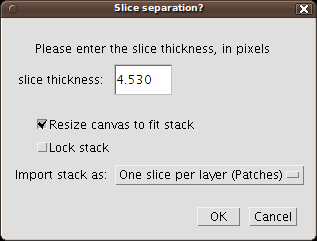
On importing a stack, you'll be presented first with this dialog:

Slice thickness: is the section thickness, in pixels. This measurement is automatically computed by multiplying the section thickness in units (like microns) by the pixel width (in pixels/micron).
To read out (and adjust) this information from the stack, open the stack by "File - Open" and then execute the menu command "Image - Properties".
Resize canvas to fit stack: when ticked, the virtual canvas of TrakEM2 will be enlarged to fit the stack inside it. If unticked, you may enlarge the canvas later by right-click on the canvas, then "Display - Autoresize canvas/Layerset".

Lock stack: when ticked, all slices of the stack are marked as locked--they cannot be dragged, rotated, scaled, etc. This is very convenient.
Import stack as: choose whether to import the stack as "One slice per layer (Patches)", or as "Image volume (Stack)". For this tutorial, choose the first option--we want one image per layer.

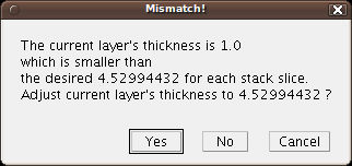
... and then with this other dialog:

By default, a TrakEM2 layer thickness is 1.0. Now, the stack to import has a larger section thickness. This dialog asks us to confirm that we change the current layer thickness from 1.0 to 4.53, the thickness (in pixels) of the stack slice.