TrakEM2 0.9a User Manual
Download the ImageJ Conference 2008 workshop paper here.
TrakEM2 © Albert Cardona and Rodney Douglas 2005--2011.
Registration machinery © Stephan Preibisch and Stephan Saalfeld 2007, 2008; Stephan Saalfeld 2009--2011.
Released under the General Public License, v2. with the exception of the Scale Invariant Feature Transform algorithm implementation, which is free only for non-commercial purposes, as is the desire of David Lowe, the inventor.
When clueless: right-click is your friend!
- Introduction
- Setup
- Create, save, open and export a project
- Introduction to modeling
- Basic usage
- Adding functionality with your own plugins
- Using TrakEM2 as a framework
Introduction
Setup
Create, save, open and export a project
Introduction to modeling
Basic usage:
- Layers and Displays: navigate, adjust dimensions, add and remove
- Add a layer
- Add a layer set
- Adjust a layer's Z coordinate and thickness
- Calibration
- Reverse selected layers Z order in one shot
- Adjust a layer set width and height
- Delete a layer
- Delete a layer set
- Navigate a layer set in a display
- Navigate a layer
- Layer overlays
- Images: importing, adjusting, transforming, reverting
- Importing single images
- Importing stacks of images
- Importing an image grid or montage
- Importing a sequence of images as a grid or montage
- Import images as listed in a text file
- Importing rare image formats such as Zeiss LSM
- Transforming images
- Reverting edited images to the original
- Color channel opacity
- Alpha masks
- Adjusting the brightness and contrast of an image by adjusting the min and max
- Correct the lens distortion present on the images
- Blend images to remove seams
- Image registration: aligning or montaging images
- Semi-automated snapping: one image onto another
- Image registration models for automatic image registration
- Montaging images automatically within a layer
- Automatic: montage images within and across layers, montage all images of a layer, and align layers
- Manual: register two layers with landmarks
- Register a sequence of layers by selected profile lists
- Profiles: create, adjust and transform
- Create a profile
- Adjust the Bézier curve
- Adjust the Bézier curve by freehand drawing
- Transform a profile
- Pipes: create, adjust and transform
- Polyline: create, adjust and transform
- Balls: create, adjust and transform
- Labels: create and edit
- AreaList: create, adjust and transform
- What is an AreaList
- Create a new AreaList
- Adjust an AreaList
- Transform an AreaList
- Merge two or more AreaList
- AreaList measurements
- Dissectors: count objects only once
- Trees: Treeline and AreaTree -- 3D skeletons with radiuses or volumes
- What is a Tree
- Create a new Treeline or a new AreaTree
- Adjust/edit/navigate a Tree
- Tag a node of a Tree
- Connectors: directional relations between objects
- What is a Connector
- Create a new Connector
- Adjust/edit/construct a Connector
- Query the connectivity graph: select upstream and downstream
- Object manipulation: select, move, link, unlink, transform
- Selecting
- Deselecting
- Move above or below one another
- Dragging
- Linking
- Unlinking
- Transforming
- Adjusting transparency and visibility
- Hide / Unhide all of a class
- Lock
- Object properties
- Deleting profiles, pipes and ball objects
- Undo/Redo transformations
- Search
Adding functionality with your own plugins
- How to run plugins on a selected image
- How to run plugins on many objects in an open display
- How to create an undo step
- How to retrieve objects when no displays are open
- How to make image snapshots of layers
Using TrakEM2 as a framework
Appendix
Introduction
What is TrakEM2?
TrakEM2 is a program to model from images. To model what is up to you.
Two different kinds of modeling concur:
- Three-dimensional modeling: objects in 3D, defined by sequences of contours, or profiles, from which a skin, or mesh, can be constructed, and visualized in 3D in programs such as Blender , Autocad, Maya, etc.
- Relational modeling: the extraction of the map that describes links between objects. For example, which neuron contacts which other neurons through how many and which synapses.
To accomplish the above tasks TrakEM2 relies on the segmentation of the objects represented in the images. That is, the outlining of each section of an object as it appears in the images, and its orderly storage in the hierarchy of existing objects.
But there's more! TrakEM2 is built on top of ImageJ, the standard in the image analysis and research community. In the graphical interface of TrakEM2, each image and its elements can be analyzed, measured, quantified and transformed with ImageJ internal functionality, and by its enormous collection of freely contributed plugins.
How is TrakEM2 different?
TrakEM2 has been designed to handle an arbitrarily large amount of images, as many as your hard drives can store.
TrakEM2 can manage large amounts of data by storing and retrieving it dynamically from a PostgreSQL database. As of version 0.3g, the program can run just as well on XML, dynamically loading and flushing images from the file system.
Why another program?
Because there is no such program out there that can:
- Handle, display, navigate, annotate, measure, transform and store a virtually infinite number of images.
- Model in 3D while generating a relational tree, the logical skeleton of the objects in a sample.
Our purpose is to perform 3D modeling in a meaningful way, not just to generate pretty pictures. We are targeting the extraction of the relational structure for the purpose of running simulations in computers, using the 3D models as a nice visualization tool for humans. We also want to compare structures to themselves and to one another across multiple experiments on similar samples.
In addition, we plan to enable distributed annotation, modeling and analysis of a large sample. The database helps in keeping data centralized and will enable, in the future, the compartmentalization of privileges in the 3D space of the sample, for multiple users to work on the same dataset without colliding with each other.
Setup
Minimal system requirements
Minimal requirements:
- Java 1.8.0 or above.
- A number of libraries, all included in Fiji.
For database projects, they are now discontinued. If you have an old project, you'll need in addition to the above:
- A PostgreSQL installation, 7.4.12 or above (8.2.* recommended).
- The JDBC postgreSQL driver.
There is a detailed TrakEM2 installation how-to.
In the real world (NOTE: circa 2007!), for handling a 300 Gigabyte project with 150,000 images, this is the computer I use:
- Intel core 2 extreme (4 cores) 2.40 Ghz
- 4 Gb DDR3 800 Mhz RAM
- 4 HD 500 Gb each, 7200 RPM, on a RAID-10 (mirrored for backup, and stripped for speed).
- Nvidia graphics card with 512 Mb or more (the more the better.)
- Ubuntu Linux 9.04 64-bit
- java 1.6.0 64-bit
- java3D 1.5.1 64-bit
The project XML template
Deciding beforehand what to model
So what do you want to model? The TrakEM2 program offers many basic object types (skeletons, areas, spheres, ...), which live at the tips of an ontology-controled tree structure for hierarchical grouping of reconstructed objects into biologically meaningful entities such as neurons, synapses, tracts and tissues. In plain language: create your own nested categories to group thousands of objects (such many "connector", each representing a synapse) into a single, and more manageable, "neuron".
When creating a new project with the command "File - New - TrakEM2 (form template)", a dialog asks for a file containing such data model (in DTD format, or as DTD inside an existing TrakEM2 XML). If you cancel the file dialog, the project is created with a root node labeled "anything". Use the right-click popup menu to rename it and add children to it.
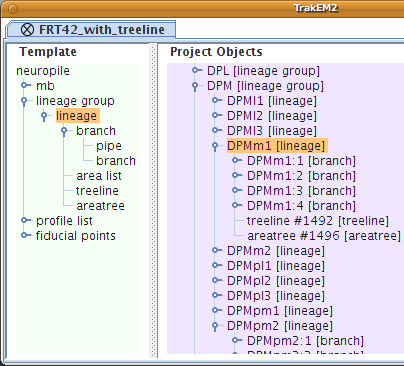
For example, if one is to model neuronal tissue, a snippet of such a template may look like (left column, in light green, titled Template):
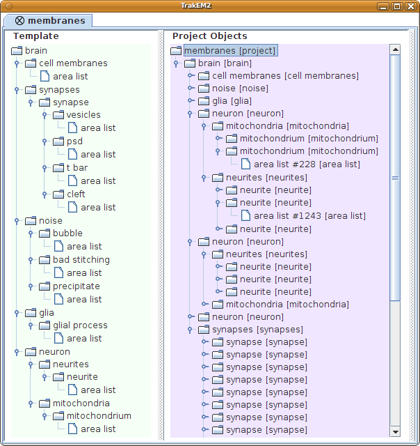
Notice the right column in light blueish: that lists the Project Objects, which are actual instances of the merely template elements of the left column. Notice how nested objects show a name "neuron" and a type "[neuron]" in brankets. The name is editable via the popup menu, or by selecting a node and typing F2.
The power of the Project Objects lays in its ability to collapse an arbitrarily large number of objects into single, parent nodes, such as "neuron", that mean something to you. This "neuron" is now the unit of control of all the objects it encapsulates, for example to select them, show them in 3D, measure them, delete them, etc.
Notice as well how some nodes have a unique ID number such as "#1243". This is the ID of an instance of a basic type object (in this example an "area list").
See example XML templates here:
- Drosophila's brain secondary lineages as DTD
- Drosophila's brain secondary lineages as XML
- Generic neuronal network (as it can be visualized in electron microscopical images)
Create and edit the template on the fly
A new TrakEM2 project can be created without any preselected XML template. The empty template tree can be filled up as the need arises, and edited any time. Use the "File - New - TrakEM2 (blank)" command.
If a template node is deleted, and there exist project objects that depend on the template, a dialog will prompt on whether to delete the project objects as well. Project objects cannot exist without a template.
Export and import a template
Once you have created a template that you find useful, you won't have to do so ever again. Right-click its root node and export the DTD file. Layer, create new TrakEM2 projects with "File - New - TrakEM2 (from template)", which will let you select the DTD file.
The basic types: area list, profile, pipe, polyline, ball, dissector, areatree, treeline and connector.
There are three basic types that can be wrapped in higher-order, abstract objects in the XML template for our sample. Briefly:
- Area Lists: a user-brushed area, flat on a section of tissue, but with multiple separated areas within the same layer and across layers.
- Profile: a user-drawn outline, bézier;-based, flat on a section of tissue.
- Pipe: a multi-point bézier curve that defines a tube, where each point is a joint that can have its independent radius, and further, can lay anywhere in the space (a pipe can cross several sections).
- Polyline: a multi-point curve that defines a skeleton across multiple sections/layers.
- Ball: a spherical object. Mostly used for small cells or nuclei at the optical level.
- Dissector: a tool to estimate object densities in space by sampling.
- Treeline and AreaTree: a skeleton made of connected nodes, which branch out. Each node holds a radius (treeline) or an area (areatree), and may have an independent color.
- Connector: a relational object that establishes directional relationships, for example to represent a synapse (one to one) or a polyadic synapse (one to many).
So before ever starting touching any image at all, the user must agree with himself and the research team on an ontology or object structure to use. In this way, the modeling flows within an enforced structure that leads to the extracting of meaningful relationships between the modeled objects.
Create, save, open and export a project
An XML file-system project
XML file-system based projects are completely independent of a database.Start a new project
Select Plugins-> TrakEM2 -> New Project, and then optionally choose a proper template file, either as a .dtd or an .xml file (the DOCTYPE declaration will be read if explicit, not an URL). If the template selection file dialog is canceled, a project with an empty (but editable) template is created.In an XML project, the original images are not saved whenever modified as in the database project. An image can always be duplicated with ImageJ's Image-> Duplicate... command (shift+d).
In an XML project you are in charge of housekeeping the images.
Open an existing project
Select Plugins-> TrakEM2 -> Open Project, and then select the XML file in which the project is contained.The images will be loaded from the proper file path entries in the XML 'patch' tags.
When images cannot be found (because for example the CD in which they lived is not mounted), an empty image with a large 'x' in the center is drawn instead.
Save and Save As
Either push 's' on a open display to save, or:- In the project tree, right-click and select "Save" to overwrite the project XML file, or push 's'.
- On a display, right-click and select "Project / Save", or push 's'.
If you'd rather save the project under a different name, select "Save As" to create a new XML file. The images are not duplicated. The new XML file points to the same image files as the original did, and the mipmaps, masks, features, etc. are shared. It's only the XML file itself that is different.
Introduction
Modeling consists of two parts: create the abstract structure, and create the basic data types wrapped in nodes of the abstract structure.
Creating the abstract structure
Creating the abstract structure is as simple as drag and drop: from the Template Tree, to the left, drag the nodes to the Project Tree, in the center. You will be prevented from dragging nodes where they do not correspond.
As a parent/child example, first create a "neuronal network" node under your Project Tree by dragging it from the Template Tree. Then drag subsequent child nodes such as "neuron", then a "soma" for the "neuron", and finally an "area list" to define the 3D volume of the "soma".
Now the next step would be to fill in the "area list" with actual areas (which are basic data types) by painting them on the canvas using the brush tool.
Creating basic data types
Filling a profile list with profiles
When reaching a basic type such as a profile, you need to have an open Display, which shows the layer in which it will be added.
Double-click on a layer to open a display for it. You can open as many displays as you want, even several for the same layer.
Navigate the layer and locate the region you want to model. You can import more images or stacks by calling the popup menu (right-click on the display) if necessary.
Go back to the trees and drag the basic type to the object you want to model. The foremost display will be brought to front, the pen tool (right-most) from the ImageJ toolbar will be selected, and all you have to do is click and drag several times on the image to create the profile, adjusting the Bézier curve as needed.
Once the first profile has been added to a "profile list", the latter cannot accept anymore profiles to be dragged into it. Instead: when done with the profile in the current layer, right-click and select "duplicate, link and send to next layer". The display will now show the next layer (notice its Z coordinate in the window title), and you can modify the profile to adjust to the new section of the object you are modeling. Iterate until the object is no longer visible in the layers.
If the object you are modeling splits in two or more profiles, go back to the previous layer where the object was still a solid, single profile and do again a "Duplicate, link and send to next layer" (or use hotkey 'n').
Now you'll have another profile to deform for the new branch.
PLEASE NOTE: as of version 0.2, the 3D models of such branched objects will fail. A proper 3D mesh extraction algorithm is on the works.
If you started modeling in a medial section, you can navigate the layers back (use the '<' and '>' keys) until reaching the first profile. Then, right-click and select "Duplicate, link and send to previous layer" (or hotkey 'b'). Proceed as a above but in the opposite direction in the volume.
When a basic object is added, the images underneath that support it become linked to it. So now, if you drag the image with the select tool (black arrow), the linked profiles will be dragged as well. And vice versa.
Adding a pipe object
Make sure a display is open. Open a display by double-clicking a layer if necessary. If no displays are open it wouldn't know which layer set to use.
Drag a pipe node from the Template Tree to an appropriate abstract object in the Project Tree, for example an "axonal branch". A display will be brought to front and you start creating the Pipe.
Adding a ball object
Make sure a display is open. Open a display by double-clicking a layer if necessary. If no displays are open it wouldn't know which layer set to use.
Drag and drop a ball node from the Template Tree to an appropriate abstract object in your Project Tree. The front most display will be brought to front, the pen tool selected, and you can start adding ball objects by clicking on the display.
Preview 3D
In the Project Tree, right-click any node and select "Show in 3D". Meshes are generated and presented in the ImageJ 3D Viewer, which must be installed (place its jar file under ImageJ's plugins folder).Work is on the way to add editing capabilities. For example, to select, measure, delete and join objects.
Exporting 3D
In the 3D Viewer, select File -> export ".obj" (Wavefront format) or export ".dxf" (digital exchange format).All meshes in the viewer will be exported.
In Blender, the three-dimensional objects can be edited and colored at will, and rendered by ray-tracing.
Basic usage
Layers and Displays: navigate, adjust dimensions, add and remove
Add a layer
A layer is a section with a given Z coordinate and thickness, both demanded at creation time.A layer exists inside a layer set. A layer set defines the width and height of the layers it contains.
In the TrakEM2 main window you'll find three trees. The one on the right let's you manage the layers and layer sets.
There are two ways to add layers:
- By right-clicking on a layer set and choosing "new Layer" or "many new layers".
- By importing a stack into a layer or a layer set. Layers are created automatically as needed.
Add a layer set
Besides the top level layer set, any layer can contain nested layer sets.In the Layer Tree, right-click a layer and select add new layer set. The new layer set dimensions will be asked for.
Each layer set has its own x,y position in the layer, while at the same time defining the width and height of the layers it contains.
The ability to nest layer sets into layers enables, for example, optical microscopy images to contain sets of sequential, electron microscopy images that were obtained from parts of the optical microscopy sections.
Adjust a layer Z coordinate and thickness
At any time, right-click on a layer node in the Layer Tree to change its Z coordinate or thickness.If multiple layers are selected (by shift+click on a second layer or control+click on any number of them), the right-click popup menu will show options to displace all selected layers in the Z axis.
To reset all thickness values to 1.0, and all Z values to the layer index, right-click on the "Top Level [layer set]" node and choose "Reset layer Z and thickness."
Calibration
Every layer (every section) in TrakEM2 has an independent Z axis position and an independent thickness. The units of the Z axis are in X,Y pixels. This requires a calibration procedure that is done in two parts: the X,Y calibration, and the Z calibration. Each is adjusted in a different part of TrakEM2.An example: suppose your volume has a resolution of 4x4x50 nanometers:
- Set the X,Y resolution by right-clicking on the canvas and choosing "Display - Calibration...". In the dialog that opens, change the units to "nm", and then change the "Pixel Width" to 4, the "Pixel Height" to 4, and the "Pixel Depth" to 50. Push ok to set the changes. (All other entries of the dialog are ignored.)
- Set the Z resolution in each layer, considering that the units are in pixels. In our example, a section of 50 nm measures 50/4 = 12.5 pixels in thickness. The Z of the next section would also be at 12.5.
- Go to the "Layer Tree" in the "TrakEM2" window.
- Right-click on the "Top Level [layer set]" node and choose "Reset layer Z and thickness". Now the first layer has a Z coordinate of 0 and a thickness of 1; the second layer has a Z coordinate and 1 and a thickness of 1, etc.
- Click on the first layer, and then shift-click on the last layer, so that all layers are selected.
- Right-click on the selected range of layers and choose "Scale Z and thickness...", type in 12.5 (50/4 = 12.5), and push ok. Now all layers will be spaced by 12.5 pixels and have a thickness of 12.5.
If your data set has a very idiosyncratic organization, for example consisting of sections of 1 micron in thickness sampled every 10 microns, and with ultrathin 50 nm sections interspersed here and there, then you may want to adjust the calibration and thickness with a script. See for example a script for "Calibrating and setting the Z dimension", written in jython.
Reverse selected layers Z order in one shot
Select more than one layer in the Layer Tree by shift+click on a second layer, or by control+click on any number of them.Then right-click and select "Reverse layer Z coords"
Adjust a layer set width and height
At any time, right-click on a layer set node in the Layer Tree to adjust the width and height of the layers it contains. The resizing operation will demand an anchor (top left, top, top right, etc.), so that the objects contained in the layers of the layer set can be placed properly according to the new dimensions.Adjust a layer set snapshots policy
Right-click on a layer set node in the Layer Tree and adjust the snapshot policy to bounding box or full snapshot. Bounding box mode is very useful to quickly navigate gigantic data sets across it's layers (Z axis).Delete a layer
In the Layer Tree, right-click and select "Delete".The deletion will not be allowed if any of the objects in the layer are linked to objects in other layers.
All the objects contained in the layer will be deleted along with it.
Delete a layer set
Absolutely all objects contained in the layers of the layer set, and the layers themselves, will be deleted.The top level layer set cannot be deleted.
Navigate a layer set in a display
A display can show you any of the layers of a given layer set. When double-clicking a layer in the Layer Tree, the display that opens will be able to browse through any of its sibling layers.To scroll through the layers in an open display, use:
- '<' and '>' keys (or their equivalent ',' and '.' keys).
- The scroll wheel.
Navigate a layer
Layers can be both zoomed and panned.Zooming:
- With the glass tool from the ImageJ toolbar.
- With the '-' and '+' keys (or equivalent '_' and '=' keys in English keyboards)
- With control + scroll wheel
- With the hand tool from the ImageJ toolbar, directly on the images.
- With the mouse, on the navigator window (lower left). A red rectangle shows the area currently displayed.
- With the middle mouse button, click-drag over the images directly - just like in Inkscape and many other graphics applications.
Layer overlays
A layer is a section containing multiple floating elements, such as images, segmentation, floating text, etc.When viewing a layer in a display, any other layer may be overlayed with a desired degree of transparency (alpha) on top of it. Just go to the "Layers" tab, scroll down to find your current layer (the panel has a green background), and then drag the alpha sliders of any othr layers you want.
Superseding layer alpha overlays is layer color overlays. When color overlays are active, the current layer is rendered in the green channel, and up to any other two layers in the red or blue channels.
To operate color overlays:
- Set a layer as red: shift+click the title of the layer in its panel, within the "Layers" tab.
- Set a layer as green: alt+click the title of the layer in its panel, within the "Layers" tab.
- Set a layer to red or green by right-click and selecting the desired color from the popup menu.
- Right-click on a layer papel to access popup menu, and reset coloring or alphas.
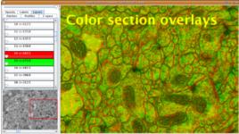 |
Movie showing how to activate/deactivate layer color and alpha overlays. |
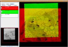 |
Movie showing the use of layer overlays in manual cross-layer registration of multiple image montages, one per layer/section. |
Create a flat image
On any display, right-click and select "Display -> Flat image". Options will be provided to create an image of the visible area or the entire layer. A regular ImageJ image window will open.The image defaults to RGB to paint properly in colors. The pixel accuracy from 16- and 32-bit images will be thus lost.
The dialog lets you select any range of layers to take a snapshot from, and also directly to an image sequence if desired. If the resulting stack is too large to fit in memory, a dialog will prompt to save the stack as an image sequence, or abort the operation.
Images: importing, adjusting, transforming, reverting, stitching
Grayscale and RGB images can coexist in the same layer. 8-bit, 8-bit color, 16-bit, 32-bit and RGB can all coexist.Each image, when selected, behaves like any other ImageJ image. Plugins and commands can be run on them.
At any point, an image can be reverted to its original state from the contextual menu.
Also, any ROI tool will work as well. Select the ROI tool from the ImageJ toolbar and create the ROI on the display. The ROI will apply to the currently selected image.
As of version 0.2 there are some limitations in ROI usage. Calling measuring and other commands such as copy/cut/paste works for some ROI types but not others. Full support is on the works.
Importing single images
Open a display by double-clicking a layer in the Layer Tree, and then right-click the display canvas.From the contextual menu, select "Import -> Image".
As of version 0.3b, these key bindings are available:
- shift+alt+i: import an image
- alt+i: import the next image in the folder, or a new image if none have been opened yet.
- by drag and drop directly into an open display. The image top left corner will be placed where the mouse was released.
If the image is an stack, you'll be asked whether to import it, creating new layers as it needs them.
Importing stacks of images
A stack is a set of images of sections consecutive in the z axis, and which have the same width and height, and usually properties (8-bit or color).There are three ways to import a stack of images:
- In the Layer Tree, right-click a layer set that contains no layers and select "import stack".
- In the Layer Tree, right-click an existing layer, and select "import stack".
- Right-click a display and select "Import -> Stack".
New layers are created on the fly to accommodate the sections of the stack, if necessary.
Whenever possible, existing layers are used.
As of version 0.3j, drag and drop image stacks directly into the canvas, or folders containing image sequences.
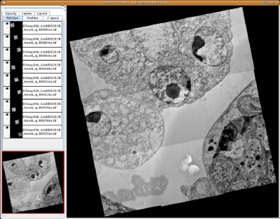
Importing an image grid or montage
An image grid or montage is a collection of images, where each image shows a part of the same section of the sample.There are three ways to import an image grid:
- In the Layer Tree, right-click on a layer and select "Import grid...". This option has the advantage that it can be performed without a display showing, i.e. when finished, there is no delay related to repainting.
- In an open display, right-click and select "Import -> Import grid"
- Drag and drop a folder of images directly into the canvas.
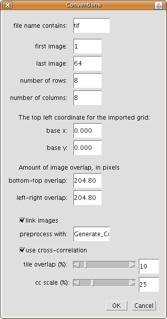
After selecting an image from a folder, a dialog will popup asking for parameters:
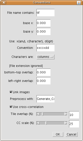
Options are:
- Filter file names in the folder by a sequence of common characters (optional).
- The top left coordinate of the grid (or montage) of images to import, i.e. the base x,y.
- The convention used to order the list of images in a grid: for each character in the image name, type in an 'x' for any character, a 'c' for character and a 'd' for digit.
- Decide whether characters specify columns or rows in the grid: for example in an image named tissue_A_002.tif, enter: 'xxxxxxxcxddd'.
- The overlap of the images on the horizontal and vertical sides. For example, if 1024 x 1024 images where taken with a 10% overlap in all directions, enter 102.4 for bottom-top and 102.4 for left-right.
- Whether images should be linked to their top/bottom/left/right neighboring images, if any (so they can be dragged as one group by dragging any of its members).
- The name of a PlugInFilter to run on every image prior to insertion. Single white space is tolerated. Any ImageJ commands or plugins that implement the PlugInFilter interface are accepted.
Note for developers: be sure NOT to multithread the plugin, for the program won't wait on it. Also, the plugin should be resistant to null images in its setup(String arg, ImagePlus imp) method, since the program tests for the existence of the plugin by invoking it with a null image. Images are passed to the plugin by simply setting the image in question as the active image in ImageJ's WindowManager (see WindowManager.setTempCurrentImage(ImagePlus) method). - Apply cross-correlation between neighboring tiles (left and top only) to correct improper overlaps. The two sliders define (1) the maximum amount of tolerated overlap, and (2)the scaling factor to apply to temporary images when cross-correlating, for speeding-up purposes.
Importing a sequence of images as a grid or montage
A sequence of images defined as image_001.tif, image_002.tif, etc., can be imported as a montage, by defining the number of columns and rows.As in importing grids, there are three ways to add them:
- In the Layer Tree, right-click on a layer and select "Import sequence as grid...". This option has the advantage that it can be performed without a display showing, i.e. when finished, there is no delay related to repainting.
- In an open display, right-click and select "Import -> Import sequence as grid".
- Drag and drop a folder of images directly into the canvas.
All images will be imported assuming they have the same size as the selected image.
Options are:
- Filter file names in the folder by the sequence of common characters (optional).
- The first and last image to use for the grid. So that for example the first half can be imported, or the last half or third, etc.
- The number of rows and columns. In the example, images 1 to 22 will be in the first row, then images 23 to 44 in the second row, etc. The number of images to import has to be exactly the product of the number of rows and columns.
- The top left coordinate of the grid (or montage) of images to import, i.e. the base x,y.
- The overlap of the images on the horizontal and vertical sides. For example, if 1024 x 1024 images where taken with a 10% overlap in all directions, enter 102.4 for bottom-top and 102.4 for left-right.
- Whether images should be linked to their top/bottom/left/right neighboring images, if any.
- The name of a PlugInFilter to run on every image prior to insertion. Single white space is tolerated. Any ImageJ commands or plugins that implement the PlugInFilter interface are accepted.
Note for developers: be sure NOT to multithread the plugin, for the program won't wait on it. Also, the plugin should be resistant to null images in its setup(String arg, ImagePlus imp) method, since the program tests for the existence of the plugin by invoking it with a null image. Images are passed to the plugin by simply setting the image in question as the active image in ImageJ's WindowManager (see WindowManager.setTempCurrentImage(ImagePlus) method). - Apply cross-correlation between neighboring tiles (left and top only) to correct improper overlaps. The two sliders define (1) the maximum amount of tolerated overlap, and (2) the scaling factor to apply to temporary images when cross-correlating, for speeding-up purposes.
Import images as listed in a text file
Right-click on a display and choose "Import - Import from text file".As simple as that: to import any number of images, list their names and X,Y,Z coordinates in a text file. The columns may be separated by space, tab or commas. Layers will be created automatically for any Z coordinate that doesn't have one already.
Image1.tif 0 0 30
Image2.tif 2048 0 30
Image3.tif 4096 0 30
...
The source folder where the images reside will be asked for.
Several parameters will be asked for, such as whether coordinates should be transformed by a defined factor; if histograms of all the images in each touched layer (as defined by the Z coordinate) must be histogram-adjusted; the thickness of the layers if they need be created; and whether all layers should be aligned when finished importing.
Importing rare image formats such as Zeiss LSM
Fiji supports just about every image file format in existence (including microscopy formats like Zeiss LSM, MRC, Biorad, etc.) thanks to the LOCI Bioformats library. If your file format is not supported, you may add support yourself by adding a new plugin to read it and adding an entry to the HandleExtraFileTypes.java file. See this tutorial here or ask the mailing list.Transforming images
The usual strategy is to use layer overlays while transforming images. To activate layer overlays, go to the "Layers" tab and set the previous or next layer as the red channel. The images in the current layer will paint in green. Then, any manual transformations on the set of selected images is done with the context of the previous or next layer.
Important: if an image or selected object is locked, you can't transform it. See it's panel in the "Patches" tab, whether it has a little lock icon in black or not. Click that lock icon to unlock or relock it.
Note that transforming images alters only their screen representation. The original images are by no means altered.
Transform images with an affine transform (translation, rotation, scaling or shear):
- Select an image or a group of images.
- Right-click and choose "Transform - Transform (Affine)" or push 't'. Both put you in affine transform mode.
- To transform the selected image or images (and any other selected objects), do any of the following:
- Drag the handles on the sides and corners to resize.
- Drag the handle by the floater, to rotate.
- Drag the floater to change the center of rotation.
- Drag anywhere with the bounds to translate.
- Shift-click to add up to three points.
With 1 point, dragging it will give you a translation, just like dragging elsewhere within the bounds.
With 2 points, dragging any of the two points gives you a similarity transform: rotation and isotropic scaling (i.e. scaling while preserving the aspect ratio of the images).
With 3 points, dragging any of the three points gives you an affine transform: rotation, scaling and shear. - Or right-click and choose "Specify transform", where translation, rotation and scaling values are entered in a dialog.
- When done:
- Push 'ENTER' to apply the transform, or right-click and choose "Apply transform".
- Push 'ESC' to cancel it, or right-click and choose "Cancel transform".
- Apply transform propagating to last layer: the transform is applied to the selected images in the current layer, but also to all the images in any subsequent layer. In this way, the relationship between the current layer and the next layer, and of the latter with its next layer, etc., is preserved.
- Apply transform propagating to first layer: the transform is applied to the selected images in the current layer, but also to all the images in any previous layer. In this way, the relationship between the current layer and the previous layer, and of the latter with its previous layer, etc., is preserved.
Important: if an image or selected object is locked, you can't transform it. See it's panel in the "Patches" tab, whether it has a little lock icon in black or not. Click that lock icon to unlock or relock it.
Transform images non-linearly:
Transforming images non-linearly works very similarly to transforming images with an affine. The main difference is that many more control points than just 3 points are possible.
- Select an image or a group of images.
- Right-click and choose "Transform - Transform (Non linear)" or push 'shift+t'. Both put you in non-linear transform mode.
- Shift+click anywhere to add a control point. Add as many as you need.
- With 1 point, dragging it will give you a translation.
- With 2 points, dragging any of the two points gives you a similarity transform: rotation and isotropic scaling (i.e. scaling while preserving the aspect ratio of the images).
- With 3 points, dragging any of the three points gives you an affine transform: rotation, scaling and shear.
- With 4 or more points, dragging a point is doing a local transformation: the other points remain where they are, and the region around the dragged point is locally transformed.
The usual strategy is to place a few points in areas that you want to preserve as they are, untransformed. These points act as anchors. Then add a few points on areas that you want to transform, and drag them.
- When done:
- Push 'ENTER' to apply the transform, or right-click and choose "Apply transform".
- Push 'ESC' to cancel it, or right-click and choose "Cancel transform".
- Apply transform propagating to last layer: the transform is applied to the selected images in the current layer, but also to all the images in any subsequent layer. In this way, the relationship between the current layer and the next layer, and of the latter with its next layer, etc., is preserved.
- Apply transform propagating to first layer: the transform is applied to the selected images in the current layer, but also to all the images in any previous layer. In this way, the relationship between the current layer and the previous layer, and of the latter with its previous layer, etc., is preserved.
Reverting images
You will almost never or never do this operation. Reverting an image means: to restore the image pixels directly from the original image.
Make sure the image is selected and then right-click and "Revert".
The original image is fetched and the screen image is replaced.
Reverting an image that is part of a stack will revert the entire stack at once.
Bear in mind that reverting an image restores its pixels, but not it's screen representation. If you have transformed the image, you can restore it's original width, height, rotation and position values values by selecting it and then right-click to adjust its "Properties...". The same is true for the alpha mask: you will have to right-click and choose "Remove alpha mask".
Color channel opacity
For RGB images, the "Opacity" tab in the display enables the control of the opacity of each individual color channel.Simply select the channel by clicking its panel, and then drag the slider.
To completely switch off a channel, select/unselect its check box.
See a sequence of snapshots.
Alpha masks
Select an image, draw with a closed ROI on top of it and push 'f'. ImageJ's foreground color will be used to fill in the mask: black means total transparency, and white total opacity.Adjusting the brightness and contrast of an image by adjusting the min and max
TrakEM2 supports setting min,max for a selected image or for all images, and also automatic histogram homogenization across selected images or for all images.
To do so, right-click and select, under the "Adjust images" menu:
- Enhance contrast layer-wise...: choose a range of layers and then enter options in the "Enhance Contrast" dialog. This is the same dialog that ImageJ and Fiji use for the command "Process - Enhance Contrast". TrakEM2 presents all images as a virtual stack to the "Enhance Contrast" plugin, hence the dialog presents options for using the joint stack histogram--but only the images of the current section are used for computing the min and max value that will be applied to each image.
- Enhance contrast (selected images)...: enter options in the "Enhance Contrast" dialog and then apply them to all images. TrakEM2 presents all images as a virtual stack to the "Enhance Contrast" plugin, hence the dialog presents options for using the joint stack histogram.
- Set Min and Max layer-wise...: a dialog pops up asking for the min, max values to apply to all images of every layer in a chosen range of layers.
- Set Min and Max (selected images)...: a dialog pops up asking the min, max values to apply to all selected images.
- Adjust min and max (selected images)...: a dialog pops up with two sliders: one for the min value and one for the max value. The little histogram is the joint histogram of all selected images, and aids in selecting the right min and max values.
If you need to get an intuitive understanding of what the min and max values mean, open any image with Fiji and then choose "Image - Adjust - Brightness & Contrast". In the dialog that opens, an histogram of the image is shown, along with 4 slides. The top two sliders control the min and max.
To learn about histograms, see Wikipedia on Image histogram.
Correct the lens distortion present on the images
Select a few heavily overlapping images. Ideally 9 images, one to be central (and selected as the active one), and among the others one image overlaps its upper half, another its lower half, another its right half, another its left half, and the other 4 each of the quarter/corners. The more overlap the better, but with only 4 or 5 images that overlap the active image from all directions could be enough.After selecting the overlapping images (and making sure the central-most image is the active one), right-click and choose "Lens correction". Choose the range of layers you want the correction to be applied to, and optionally tick the checkbox to output as well an image representation of the deformation model.
All images must be of the same dimensions, i.e. identical width and height. Otherwise the model cannot be estimated correctly neither applied properly.
For all details on how the lens distortion correction works, see Verena Kaynig's PDF documentation in the Fiji wiki.
Blend images to remove seams
Select the images you want to blend together. If the images don't overlap, they won't blend (obviously!)The stack order, i.e., the overlapping order of the images will determine the blending: images on top will blend onto the images under them.
The blending modifies the alpha mask of the mipmaps, using the same formula from Stephan Preibisch's stitching plugins.
Before and after (notice the borders between images):
 |
 |
If the seams are too severe because the contrast differences are too big, you'll have to preprocess the images. A proper API to do so is on the works.
Image registration: aligning, montaging or stitching images
Semi-automated snapping: one image onto another
An image dragged onto another can be snapped to it by pressing alt+s while dragging, or right-click and select 'snap'.A subset of the pixels will be analyzed for similarity on both images and then the dragged image is displaced for an optimal match.
When more than one image lay under the dragged image, the dragged image is aligned with the best matching image.
It is much better to use the montage function.
Image registration models for automatic image registration
- Translation: only displacements in X,Y.
- Rigid: translations plus rotation.
- Similarity: translation, rotation and isotropic scaling (that is, it preserves image aspect ratio.)
- Affine: free affine transform, which amounts to translation, rotation, scaling, and shear.
When your collection of images contains images acquired at different resolutions, select one image to act as reference (or lock it), and then apply a similarity model for both feature extraction and alignment (the "expected" and "desired" transformations, respectively.)
In the near future, elastic and moving least squares models will be supported.
Feature extraction parameters (initial gaussian blur, steps per scale octave, minimum image size, maximum image size, feature descriptor size, feature descriptor orientation bins, closest/next closest ratio, maximal alignment error, inlier ratio, expected transformation, and desired transformation) are explained in Fiji's Feature Extraction wiki page.
Montaging images automatically within a layer
Select 2 or more images and right-click to choose "Montage".The "Montage" menu entry appears only when 2 or more images are selected.
If images are linked to segmentations, montaging is not possible.
Keep in mind that this is just one of the many image montaging options; see below.
Montage images within and across layers, montage all images of a layer, and align layers
Right-click on a display to bring up the popup menu, and go to "Align" submenu:- Align multi-layer mosaic registers all images from a selected range of layers, by finding correspondences between images within a layer and with the previous and next layers. A global optimizer minimizes the global interdistances.
The relative position of images within a layer is altered by this method.
When using a similarity or affine model, to correct for example for image resolution differences or small image scaling problems, select one image to act as reference (or lock it), i.e. an image that will serve as the scale reference you want all other images to register into. Otherwise one may be chosen at random.
The "deform" checkbox will apply a non-linear coordinate transform to the images after applying the as-rigid-as-possible optimization of the multi-layer montage, removing jitter substantially. - Align layers registers whole layers, as they are, one to another. A dialog lets you choose the range of layers that you want to register one to another, along with feature extraction parameters.
This method works by taking an image snapshot of each layer and performing the reigstration based on that. The relative position of images within a layer is not altered.
The current layer will be left untouched; the registration will proceed towards any choosen layers before the current layers, and towards any choosen layers after the current layer.
For other layers not included in the range, you can transmit to them the registration applied to the nearest rgistered layer by ticking in "propagate". This will preserve any previous layer registrations you may have done.
There are three methods:
- Least squares, linear; based on SIFT correspondences extracted on a snapshot of the minimal rectangle containing all visible images in the layer. See an explanation of the SIFT parameters.
- Non-linear based on an initial least squares (like above) and then applying forward non-linear transforms with bUnwarpJ (non-linear cubic B-splines). Use only for short series; in general it's better to use the elastic spring-mesh approach (see below).
- Non-linear elastic spring mesh based on block-matching features. The most powerful, it is able to match the current section with several sections before and after, thus being nicely regularized and very resistant to noise and missing sections. Should be your preferred method for everyday use. See an explanation of the parameters
- Align stack slices registers the slices of an imported image stack. Since slices of a stack are linked to each other--to represent the known relationship between them--, stacks require this specialized registration method. Stacks cannot be part of other registration methods because of their interlayer image links.
- Align layers manually with landmarks enters a manual alignment mode, in which clicking on the display adds a new landmark (remove it with shift+control+click as usual). Then browse to next or previous layers and add landmarks as well in the same order and the same number of landmarks in each layer. Then browse to the layer with landmarks that you want to use as reference, then right-click and choose how to apply the registration (propagating to other layers or not, or cancel it)
- Montage all images in this layer does what it says and it's equivalent to selecting all images in a layer and choosing "Montage..." from the right-click popup menu. All three approaches are available (see below in "Montage selected images"). Keep in mind that any locked or selected image will NOT be moved, but will serve as reference to the others.
- Montage selected images
- Phase correlation of the image tiles with their overlapping neighbors (only translation). Very fast but very limited and error-prone in the presence of noise or deformations.
The "tile overlap" parameter is used as the initial guess (for performance reasons; automatically uses increasingly larger chunks of the images on failure) and the "scale" indicates at which magnification to do the phase correlation (again for performance reasons; lower magnification is way faster). - Linear transformation models (translation, rigid, similarity and affine) estimated from SIFT correspondences. Reasonably fast and accurate when non-linear deformations are not severe. See an explanation of the SIFT parameters.
- Elastic spring-mesh transformations based on block-matching correspondences. See an explanation of the parameters. Reasonably fast and very accurate; and so far able to fix even lens deformation models and any kind of heat-induced section deformations that we have thrown at it.
- Phase correlation of the image tiles with their overlapping neighbors (only translation). Very fast but very limited and error-prone in the presence of noise or deformations.
- Montage multiple layers montages all images in every layer of a chosen range of layers, independently for each layer, using one of of the three methods available (see "Montage selected images" above). It's the equivalent of doing a "Montage all images in this layer" by hand on every chosen layer.
Register two layers with landmarks
- Start by entering manual registration mode, by right-clicking and choosing "Align - Align layers manually with landmarks".
While in manual registration mode, zooming and panning works as usual. - Pick the select tool (the black arrow) to add landmarks.
- Click on conspicuous points on any of the images within the canvas. There must be the same number of landmarks in both layers. Notice how each landmark is numbered: the numbers have to match across layers.
- When done, right-click to see various options, or:
Push 'ESC' to cancel (and exit the manual registration mode, loosing the landmarks)
Push 'ENTER' to register all images and their linked objects.
Important: you may register 2 or more layers in one shot, but the layer in which you push 'ENTER' will be left untouched. It's the other layers that get registered to it.On the right-click menu, there are the following options:
- Apply transform: just like pushing the 'ENTER' key, all layers are registered to the currently visible layer.
- Cancel transform: exit the transformation mode, losing any manually entered landmarks.
- Export landmarks: save all manually entered landmarks to an XML file.
These landmarks are project specific, and are stored in absolute coordinates.
If you remove a layer, later on when importing lanmarks, the landmarks for that layer will be ignored.
If you resize or alter the dimensions of the canvas (in particular, the position of the top left corner), the landmarks will get reimported in the wrong place. - Import landmarks: import all manually entered landmarks from an XML file.
Register a sequence of layers by selected profile lists
First open a display and select as many profiles as you want to use, each potentially belonging to its own profile list. Use shift+click with the black arrow tool selected to select more than one, or just shift+click over the left panel on the profiles' tab.Then select the alignment tool, and right click on the display and select "Align using profiles". The entire contents of all layers will be affected.
All layers where the involved profile lists have profiles will be aligned using consecutive profile pairs as landmarks. When no profiles exist for a layer, the proper transformation will apply relative to transformations in other layers.
You can always undo the transformations.
Profiles: create, adjust and transform
Create a profile
Make the layer you want to draw the profile into be displayed in the front most display. You can either double-click the layer from the Layer Tree to open a new display for it, or navigate your current display until finding it.Drag a "profile" node from the Template Tree to a "profile list" node in the Project Tree. If the "profile list" already contains one profile, you must continue from that profile by selecting it and then right-click and select "Duplicate, link and send to previous/next layer".
The first point of the profile defines the layer in which it will exist.
Click and drag on the display, anywhere over the edge of the structure to outline. Drag towards where you are going to set the next point.
Now click and drag towards the previous point. The curve is drawn, and while dragging towards the first point the curvature is adjusted.
Proceed clicking and dragging towards the previous point.
Finally, shift+click on the first point and drag towards the last, to close the curve while adjusting the curvature of the last segment.
All points can be dragged together by alt+drag on the area enclosed by the curve.
Toggle the closed state of a Profile with shift+c.
Adjust individual points in the Bézier curve
Select the pen tool from the ImageJ toolbar, if not already selected.At any time, click and drag over the curve to insert a point between two existing points.
Shift+click any point to toggle the open/closed state of the curve.
At any time, click and drag the handles of any point to adjust the curvature.
Also, alt+drag a point to reset its handles.
To drag a point and its handles, simply drag the point.
To delete a point, shift+control+click it, or push 'x' to delete all points in the profile.
Adjust the Bézier curve by freehand drawing
New in version 0.3g
Select the pencil tool (the one on the left of the pen tool) in ImageJ's toolbar
. Click and drag on a point to draw freehand. Release the mouse to finish. The curve will close on the nearest point.
The slower the movement of the freehand the more bézier points will end up making the profile.
A profile can be drawn from scratch using this technique, no points need to exist beforehand.
[This functionality contributed by Mathias Buehlmann]
While the profile is unlinked (either it has not been deselected yet, or it has been actively unlinked), you can drag the whole curve with the black arrow tool.
Transform a profile
Make sure the profile is selected. When selected, the profile will show its points and control points besides the curve itself.
With the pen or the black arrow tool selected, push 't' or right-click and select 'Transform'. The bounding box will be drawn, with handles to deform it.
Pull the handles with the mouse to deform the profile. When done, push ENTER to accept, ESCAPE to cancel, or right-click for these options and also to enter a specific transform.
Cancel the transformation anytime by pushing the ESC key.
Pipes: create, adjust and transform
Create a pipe
Make the layer you want to start drawing the pipe into be displayed in the front most display. You can either double-click the layer from the Layer Tree to open a new display for it, or navigate your current display until finding it.Drag a "pipe" node from the Template Tree to an abstract node in the Project Tree that can contain it. You can proceed to add points by click-drag, adjusting the bézier curve, and then shift-drag, to adjust the radius of the pipe at that point.
Navigate the layer set back and forth following the structure (an axon bundle, a dendrite) that you are modeling with a pipe. Add points to the same pipe in any layer.
The segments of the pipe resident in the layer will be linked to the images underneath, over which the pipe was drawn.
Adjust a pipe
Pipes exist in the entire layer set, not just in the current layer. Thus, only those pipe sections showing in the current layer are editable.The pipe is a Bézier curve, and thus pipe points and control points can be adjusted like those of a profile, three differences withstanding.
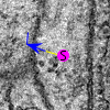
First, a pipe cannot be closed. Second, the points of a pipe can exist in different layers. The segments of a pipe that exist in previous layers are painted in red, while those existing in deeper layers are painted in blue (see snapshot).
The points of a pipe that exist in the current layer are painted in the pipe's color.
Third, pipe points have a radius: by shift-drag on a point, you can increase and decrease the radius of the pipe at that point.
The radius of a new point is determined by the radius of the point that precedes it, unless manually edited.
Points in the current layer can be added either by insertion (click-drag near the medial line of the pipe) or by clicking anywhere, in which case they are appended at the end.
In summary:
- Click+drag to add a point and extend the control points symmetrically.
Can be done at the beginning (prepend), at the end (append), or inserting in between (click+drag over a segment of the pipe.) - Shift+drag on a backbone point to adjust the radius of the pipe.
- Alt+drag on a backbone point to adjust both control points symmetrically.
- Click+drag on a control point to adjust it.
- Shift+control+click to delete a point.
- Push 'p' to toggle the painting of color cues (red for segments in previous layers, and blue for segments in subsequent layers.)
While doing all the above, use the scroll wheel to navigate through layers, control+wheel to zoom in and out, and middle-click+drag to pan the view (so you don't need to change to the glass and hand tools to do that.)
When done, push ESCAPE key to deselect the pipe, and thus prevent accidental addition of points.
Transform a pipe
Just push 't' on a selected pipe, or right-click and select "Transform". Then push 'ESCAPE' to cancel, or 'ENTER' to accept. Or right-click and select cancel or accept or entering of a specific transform.Polyline: create, adjust and transform
Create a polyline
A Polyline is a list of points that exist througout all layers.Segments of the polyline above the current layer paint in red, and segments below paint in blue (toggle color cues with 'p'). Segments within the current layer paint in the polyline's color, adjustable from right-click menu "Properties" or by clicking on ImageJ's color palette when a polyline is selected. Double-click the Dropper Tool in ImageJ toolbar to open the color palette.
Drag a "polyline" node from the TemplateTree to an abstract node that can contain it in the Project Tree. Then proceed to use the Pen Tool to add and manipulate points, or the Pencil Tool for semi-automatic tracing.
Adjust a polyline
Push 'p' to toggle the painting of color cues (red for segments in previous layers, and blue for segments in subsequent layers.)With the Pen Tool:
- Click to add a point. Will be appended to the end, or prepended to the beginning depending on proximity.
- Drag a point to move it.
- Shift+Control click to delete the point nearest to the click.
- Push 'p' to toggle the painting of color cues (red for segments in previous layers, and blue for segments in subsequent layers.)
- Click to start a semiautomatic tracing towards the last added point. Adds a point if there are none.
- Drag a point to move it.
- Shift+Control click to delete the point nearest to the click.
- Push d to delete the last set of autotraced points. Careful: if you edit any points within this set, or add/delete more points on this end of the Polyline, you would not be able to delete the last set of autotraced points -- since it would delete user-edited points.
- Push r to delete the cached data for tracing (such as the Hessian matrix, virtualization scale, etc.) Which is done automatically anyway when adjusting the virtualization scale (from right-click "Display - Properties" dialog).
Transform a polyline
Just push 't' on a selected pipe, or right-click and select "Transform". Then push 'ESCAPE' to cancel, or 'ENTER' to accept. Or right-click and select cancel or accept or entering of a specific transform.Semiautomatic tracing
As described in adjusting a polyline, the Freehand Tool may be used for semiautomatic tracing. TrakEM2 uses the Simple Neurite Tracer by Mark Longair as a library (Update: nowadays the SNT with many contributions from Tiago Ferreira).A mini-howto:
- Select the Freehand Tool (looks like a pencil).
- Click on a bright part of an image. For example, on a GFP-labeled neurite appearing white on a black background.
- Click again farther into the neurite, and wait: a task is in motion to automatically trace the most probable line. (To navigate effectively, use the scroll wheel to move between layers, the middle-click to pan, and control+scroll wheel to zoom in and out).
- If you don't like the autotrace, push 'd' to erase it. Then click closer to the last point, which increases likelihood of success.
- Go back to point 3 to continue until done.
You can import multiple stacks, one next to another, and the autotrace will work just fine across them -- except if you have gross contrast differences (if so, I recommend using Stephan Preibisch's Stitching plugins, included in Fiji, to generate nice, smoothly blended and stitched stacks from multiple source stacks. Then import the resulting stack instead of each individually.)
Since the Simple Neurite Tracer requires the entire stack to trace into present in the RAM memory, so one may run out of it when the stacks are large. The maximum dimensions of the input stack are controled via the right-click menu, at the "Display - Properties" dialog. Just be sure to make it small enough.
Balls: create, adjust and transform
Create a group of balls
A ball object is composed of many individual balls. The ball object is thus a group of many balls.Drag and drop a "ball" node from the Template Tree to a node in the Project Tree that can contain it. A display needs to be open just as with profiles and pipes.
Each ball is represented by a triple x,y,z coordinate plus a radius. In the display, click anywhere to add a ball, or shift-click to add while adjusting its radius. Any subsequent balls will have the radius of the previous.
Navigate the layer set and add individual balls in any layer. Just like the coloring hints in pipes, balls existing in the immediately previous layer are colored in red, and those in the immediately next layer in blue.
This hints help in avoiding the repetition of balls that show partially in two consecutive layers.
Adjust individual balls
At any time, while a ball object is selected (will be labeled orange in the Project Tree, and with a blue background in the "Z space" tab), you can use the pen tool to add more individual balls.Any ball in the current layer can have its radius be edited by shift-drag.
Delete an individual ball by control+shift+click, same way you would delete points for pipes and profiles.
Transform a ball
At any time, the entire ball object can be transformed by pushing 't' or right-click and "Transform", and transformed by dragging the bounding box handles. The radius of the balls will be scaled along. Push ESCAPE to cancel, ENTER to accept, and right-click for these option and also to specify the transform.Labels: create and edit
Create a new label
Labels are independent of the Project Tree. You can create a label anytime anywhere.Labels will also become linked to the underlying images when deselected, and they can be unlinked to be dragged elsewhere.
To add a label, select the Text tool from the ImageJ tool bar and click anywhere on the display. Enter as much text as you want in the window that opens.
When done, close the window. Only the first 10 characters or the first word will be painted on the screen.
While selected, the label background will be highlighted in a contrasting, semi-transparent color.
Before adding the label, the text font, size and style can be selected from the dialog opened by double-clicking on ImageJ's text tool.
Edit/Read a label
Labels can be read in full, and edited, by double-clicking them while selected. A text window will open, with the title set as that of the label. You can have as many open as you need.Clicking an existing label with the Text tool will also open its text window for editing.
To edit the font family, size and style, right-click and select "Properties". See options at the bottom of the dialog.
Adjust/move/colorize a label
When unlinked, or not yet deselected for the first time, labels can be dragged with the black arrow tool just as any other floating object.While selected, clicking on the color picker window will change the color of the text.
To adjust the font, size and style, right-click a selected label and choose "Properties".
AreaLists: create, adjust and transform
What is an AreaList
An AreaList consists of a number of painted areas anywhere on the entire layer set.An AreaList exists in the entire layer set, not just in the current layer. So feel free to paint anywhere, while scrolling through the layers.
Create a new AreaList
First create a template object that contains an AreaList. As easy as right-clicking on any node in the Template Tree (leftmost tree) and selecting "new / area_list".Once a template exists, create as many instances of it as you need in the Project Tree. Simply by drag and drop, or right-click on the appropriate node in the Project Tree and select "new / area_list".
The "Brush" tool
 tool will be selected, the display will come to the front and the new AreaList will be selected (blue background) under the Z-space tab.
Like any other objects, the AreaList will become linked to any underlying images both when deselected and when scrolling through layers.
Adjust a new AreaList
See a video on how to segment with arealists, which covers part of what is listed below.Be sure to have the "Brush" tool
tool selected in ImageJ's toolbar (mouse over a tool will tell you its name), then:With the left mouse button:
- Drag to paint.
- Alt+drag to erase.
- Shift+click to fill a hole. If the click is in a hole of another arealist object or the hole defined by the overlapping contours of several arealists, the hole is filled as well.
- Shift+alt+click to erase a filled area.
The diameter of the brush is adjusted by either of:
- Shift+scrollwheel.
- Double-click on the oval/brush ROI tool, and adjust the brush value.
- 'f' to fill all holes (within current layer only).
- 'c' to copy the area in the current layer of the selected area list.
- 'v' to paste last copied area to the area of the current layer of the selected area list. Works across layers and across different arealists.
- 'a' to add the area defined by the current closed ROI, if any, to the area of the selected arealist.
- 'd' to delete the area defined by the current closed ROI, if any, to the area of the selected arealist.
- 'k' to part/separate the area clipped by the current closed ROI, if any, to a new area list object, which is added as a new node next to the source arealist in the Project Tree.
- 'x' to delete the whole set of areas in the selected area list, within the current layer only.
- 'm' to move the area or areas within a layer. Push 'm', then click inside the area with the brush tool and drag it. Upon releasing the mouse, the area or areas are set in place.
Painting modes:
- Overlap: multiple arealists can coexist in space (the normal mode; arealists are independent.)
- Exclude: when painting in an arealist, do not allow paint to ocurr over any other existing arealist.
- Erode: when painting in an arealist, paint in the current but erase any other arealist.
- Direct click: starts up a task fill, by fast marching, the "inside" of the region/color meseta. Uses Erwin Frise's Level Sets library.
- Control+drag: lasso tool.
Fast-marching region growth and lasso tool are both constrained to the visible XORed rectangle around the mouse. To enlarge/shrink the box, use shift+scroll wheel while using the PENCIL tool.
Be sure to check the "Display - Adjust fast-marching properties..." dialog for the settings of the region grower. These settings can also be adjusted in the "Tool options" tab to the left of the Display.
In addition, right-click and choose "Properties" from the popup menu to adjust several values, including an option to paint the AreaList as outlines instead of as filled areas.
See a video on how to segment with arealists.
Transform an AreaList
Make sure the AreaList is selected and then push 't' or right-click and select "Transform" from the popup menu. Right-click to accept, cancel or specify a transform. Also ENTER to accept and ESCAPE to cancel.Any linked objects will be transformed along with the AreaList.
Merge two or more AreaList
Select as many AreaList objects as you want, and right-click and choose "Merge" from the popup menu.The active object in the selection will be kept as a base onto which all others are merged. Superfluous, empty parent nodes in the Project Tree will be removed.
AreaList measurements
The volume of an arealist is estimated as the area within a section times the thickness of a section, plus the difference in area between the areas of two consecutive sections times the thickness and divided by 2.The surface of an arealist is estimated in its lower and upper bounds, and the average of both. The surface measurement is estimated from the areas and the perimeters; hence, the "UBs-surface" (Upper Bound smoothed surface measurement) has the perimeter smoothened out, to avoid overstimating it--since the painted areas have only integer precision. The "UB-surface" (Upper Bound surface measurement) computes the perimeter as is, directly from integer-precision painted areas.
For a graphical understanding of upper and lower bound surface estimation, see figure below:
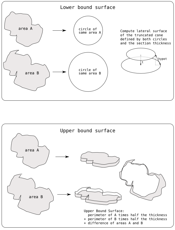
The maximum diameter of an arealist is estimated as the maximum distance between any two contour points in 3D space.
Dissectors: count objects only once
What is a Dissector
A 'Dissector' is a technique for counting only once objects that appear in multiple sections of a three-dimensional tissue. There are numerous variants. The Double Dissector technique, along with detailed statistical analysis detailing when to stop counting, how to sample a large dataset properly, etc., is explained in this paper:Geinisman, Y., Gundersen, H.J.G., van der Zee, E. and West, M.J. 1996. Unbiased stereological estimation of the total number of synapses in a brain region. Journal of Neurocytology 25:805-19.
Create a new Dissector
First create a template object that contains a Dissector type. As easy as right-clicking on any node in the Template Tree (leftmost tree) and selecting "new / dissector".Once a template exists, create as many instances of it as you need in the Project Tree. Simply by drag and drop, or right-click on the appropriate node in the Project Tree and select "new / area_list".
The PEN tool will be selected, the display will come to the front and the new dissector will be selected (blue background) under the Z-space tab.
Like any other objects, the Dissector object will become linked to any underlying images both when deselected and when scrolling through layers.
Adjust/edit/construct a dissector
A dissector object consists of a group of items to count, each item consisting of a set of marks in consecutive layers, at a reason of a mark per layer.
When scrolling through layers, marks in the previous layer appear in red, and marks in the next layer appear in blue. Such color hints enable you to know where have you added already a mark in the previous and/or next layer, and thus whether a new item should be added, or just a mark for an existing item.
Be sure to have the PEN tool selected in ImageJ's toolbar (mouse over a tool will tell you its name), then:
With the left mouse button:
- Click outside any existing marks to add a new mark, starting a new item to count.
- Click on the red or blue ghost of a mark to add a new mark for that item.
- Drag to move a mark.
- Shift+drag a mark to resize all marks for an item.
- Shift+control+click to erase a mark.
[click to enlarge]
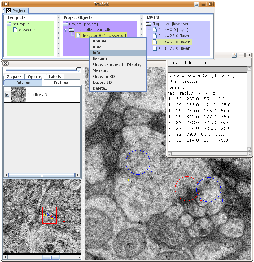
Analyze a dissector
All information regarding a dissector is obtained by right-click on it's project node and selecting 'Info'.A text window will open containing the number of items counted, and then a detailed list of all marks for all items. The data list is spread in columns for easy processing in a spreadsheet.
To measure the area of a dissector, use the Rectangular ROI tool (leftmost tool in ImageJ's toolbar) and then push 'M' or Analyze -> Measure. If you had calibrated the project first (with Analyze -> Set Scale), then the measured area will be given in microns, meters, or any units you entered.
Eventually statistical tools will be built in.
Trees: Treeline and AreaTree -- 3D skeletons with radiuses or volumes
What is a Tree
A Tree is a set of interconnected nodes, where nodes are hierarchically related to each other, and each node may have multiple children nodes but only one parent.
Three-dimensional structures like neuronal arborizations may be modeled with either of Treeline or AreaTree types, both a kind of Tree.
Four kinds of nodes:
| 1. A single root node: a node without a parent. |
 |
A root node is labeled with "S" for "Start" or "Source". |
| 2. Any number of slab nodes: nodes with one parent and only one child. |
 |
A slab node is labeled like a point in a polygon ROI. |
| 3. Any number of branch nodes: nodes with one parent and more than one child. |
 |
A branch node is labeled with "Y". |
| 4. Any number of end nodes: a node with a parent node and without children nodes. |
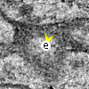 |
An end node is labeled with 'e' for "End". |
Properties of nodes:
- Nodes in the tree may sit at arbitrary layers, i.e. each node may have a different Z coordinate.
- Nodes are connected by edges, and the edge has a confidence value from 0 to 5.
- 0 is minimum or no confidence
- 5 is maximum or total confidence.
The confidence of the relationship between a child node and its parent
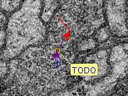
expresses how sure one is that the tree continues in that direction. - Nodes may have any number of tags: text labels such as "TODO", "Uncertain end", etc., user-defined.
Tags are searchable within the "Search" window (open it with control+f).
There are two Tree types:
| Treeline: A tree whose nodes have a radius. Every node may have its own radius. Any new node inherits by default the radius of its parent node. Adjust the radius with shift+alt+drag or shift+alt+scroll wheel on the node. In 3D, the Treeline appears as a series of connected tube segments, with the skeleton inside. |
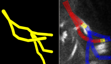 |
|
| AreaTree: A tree whose nodes may have an associated area (paintable with the brush, like in AreaList). In 3D, the AreaTree appears as an arbitrary volume (generated with marching cubes like AreaList), with the skeleton inside. |
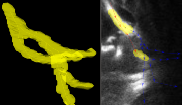 |
|
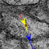
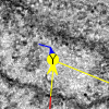
Color cues: notice how part of the trees are in red and parts in blue:
- Red indicates parts of the trees before the current section, i.e. towards the first section.
- Blue indicates parts of the trees beyond the current section, i.e. towards the last section.
The number of sections to color cue is adjustable in the right-click "Display - Properties..." dialog. Type in "-1" to color cue all sections. Otherwise, a setting of "2" means that the two sections before the current section are painted in red, and the two sections after are painted in blue.
The parts in yellow in the above pictures are the parts of the tree within the current section. Yellow happens to be the default color for a newly created object.
Create a new Treeline or a new AreaTree
To create a new Treeline or AreaTree:
|
|
 . Then:
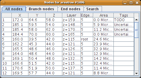
To tag a node:
The ESC key will cancel a tagging operation. If a key doesn't have a tag associated with it, a dialog asks to add one first. Then the node is tagged with it. |
|
| If you want to define a new tag for a key that already has a tag associated with it, push 't' then '0' (zero) and then the key. A dialog pops up to associate another tag for that key. Then, on pushing 't' and that key on a node, a popup menu presents the list of possible tags for that key. Notice the numeric accelerators: push the number to choose that key. |
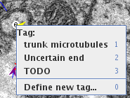
|
Use right-click "Export - Tags..." to export an XML file containing all tags.
Use right-click "Import - Tags..." to import an XML file containing manually defined tags, or exported from another TrakEM2 project.
Connectors: directional relations between objects
What is a Connector
A Connector consists of an origin point and any number of target points.
A connector can express, for example, a synapse, or a polyadic synapse.
The origin point and the target points are like pins. Any objects containing the origin point are then related, via the connector, to any objects under the target points.
A point is sufficient to capture an area of an AreaList or an AreaTree. But to capture a node of a Treeline, or a point of a Polyline, extend the radius of the origin and target points to enclose the tree node or polyline points.
|
Connector object representing a polyadic synapse in the Drosophila larval brain. Its origin point has a broad radius that encloses the node of a Treeline. Its multiple target points have smaller radiuses, one of which encloses a Treeline corresponding to another traced neuron. |
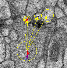
|
|
Next section, showing color cues for the same connector object. Red indicates that the origin and some targets are in the previous section. Blue indicates that there is still yet another target but in the next section. Color cues reach only the next and previous sections. The edge connecting the origin point and a target point may paint only its proximal or distal half, accordingly. |
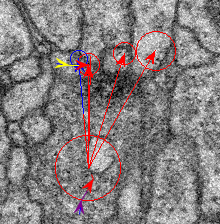
|
Connectors are also trees
Connectors can have:
- their radiuses adjusted
- their node color adjusted
- their nodes support text tags
... just like a treeline.
Create a new Connector
Follow the same instructions for adding a new object to the "Project Tree", as described for Treeline and AreaTree
Adjust/edit a Connector
- Click to add a point. The first point is the origin. Subsequent clicks are the targets.
- Move a point by dragging it with the mouse.
- Shift+drag a point to adjust its radius.
- Shift+control+click a point to delete it. If you delete the origin, the whole connector object is deleted (it asks for confirmation first).
Query the connectivity graph: select upstream and downstream
Select first one or more objects, such as a Treeline, an AreaTree, a Polyline, an AreaList, etc.
Then right-click and choose "Selection - Graph" and any of its submenu items.
- Select outgoing Connectors: add to the selection all Connector instances whose origin intersects with selected object(s).
- Select incomming Connectors: add to the selection all Connector instances whose targets intersect with selected object(s).
- Select downstream targets: add to the selection all objects that intersect with connector targets, for connectors whose origins intersect with selected object(s).
- Select upstream targets: add to the selection all objects that intersect with connector origins, whose targets intersect with selected objects(s).
The above commands provide the means to, for example, select all connectors that represent the presynaptic sites (origins) of a specific neuron, modeled with a Treeline.
Right-click and call "Show in 3D" to see the local neural network.
Successive calls to any of the above commands increases the selected network in one or the other direction (higher-order or lower-order), making it then easy to visualize or manipulate entire series of network levels.
Object manipulation: select, move, link, unlink, transform
Selecting
Select a profile, image, etc. by clicking it with the black arrow, or selecting it from the list under the proper tab to the left of the display window.Alternatively, you can shift+click on a profile, image, etc. and make a multiple selection.
- Click to select
- Shift+click to add to a selection
- Shift+click a selected object to make it the active object in the selection
- Shift+click the active object in a selection to deselect it
If more than one object exists under the clicked point, a popup will list all the possible selectable objects from which you can choose the profile.
When selected, profiles, pipes and balls will be highlighted in the Project Tree.
Any selected object will be shown in the proper display tab, with its background in blue (if it's the active object) or in pink.
The Display has a popup menu with a Selection submenu: in there you may select all (ctrl+a), select none, select by type and select all under ROI.
Deselecting
Push the ESC key to deselect all.Otherwise, shift+click with the SELECT tool (black arrow) a selected and active object (has a white frame) to deselect it.
Selecting an object other than the selected one will also deselect the currently selected object(s), unless it's shift+clicked.
Move above or below one another
Floating objects within the same layer can overlay one another. The order in which they overlay each other can be changed.The contextual menu either over the selected floating object or over its snapshot panel provides entries to move up, down, top and bottom.
As of version 0.3b, these key bindings are available:
- Home: move to top
- Page up: move up
- Page down: move down
- End: move to bottom
Dragging
Once and object is selected, you can drag it with the black arrow tool.If the object is linked to images, and thus maybe indirectly to other objects, the entire group of linked elements will be dragged together.
When working with stacks, the linked group includes objects in other layers. That is, the other images in the stack and any other object linked to them.
Non-image objects can be unlinked and then dragged independently.
Linking
Linking is automatic.Linking is the binding of a floating object to an image, or an image to another image. For example, the moment a profile is unselected it becomes automatically linked to whatever images lay under it, in that layer. The same speaks for labels, pipes and balls.
What linking means is: the floating object is supported by the image to which it is linked.
That is why linking occurs: if it didn't, the moment an image or a profile was dragged from its position, it would become meaningless.
Links are also used to preserve pre-knowledge on the arrangement of images:
- When importing a stack, all images are chain-linked, that is, every slice is linked to the next.
- When importing a grid or montage of images, options are given to link each image with its immediate neighbors.
In any case images within the same layer can be indirectly linked to each other if a floating object, for example a profile, is draw over both.
Unlinking
All floating elements in a Layer can be unlinked. The images, if linked to other images because they are part of a stack, cannot be unlinked (would be meaningless and would introduce artefactual relationships between data).To unlink, simply select the object and right-click. From the contextual menu select "Unlink". The object will remain unlinked until it becomes deselected (another object is selected, or ESC is pushed, or an empty area of the layer is clicked).
Transforming
Any floating object, including images, can be selected and then transformed by pushing 't' or selecting "Transform" from the right-click menu, with the black arrow tool selected.While transforming, selected objects cannot be transformed in any other display.
While transforming, selected objects are drawn with their compound bounding box and a set of handles that are used to stretch and deform it.
Drag the center of rotation elsewhere before rotating if desired.
In addition, you may shift+click up to 3 points to achieve:
- 1 point: just translation, like clicking and dragging within the box.
- 2 points: similarity transform, i.e. isotropic scaling.
- 3 points: free affine transform.
To remove a shift+clicked point, shift+control+click it.
Manual transformations are best used for manual section registration in combination with layer overlays; activate the layer overlays anytime from the "Layers" tab.
Push the ESCAPE key to cancel a transformation.
Push ENTER to apply the transformation.
Alternatively, use the contextual menu (right-click) to apply or cancel a transformation.
The contextual menu has further options, such as to apply propagating the transformation to all layers before or after the current one. This functionality is very useful when manually registering one layer that didn't get registered properly by automatic means.
Transformations are most powerfully used in combination with the undo.
The data is not transformed, only its screen representation via the modification of an affine transform.
Movie on creating a montage automatically and then manually registering two montages, one per section, using layer overlays and manual transforms.
Adjusting transparency and visibility
Any floating object can be set transparent, or totally invisible, whenever convenient.When the object is selected, drag the slider to adjust its transparency.
In its proper tab, set the check box selected or unselected to make the object visible or invisible, respectively.
The transparency is preserved when the visibility is toggled with the check box.
As a convenient shortcut for manual montaging, select an image and push the space bar to set its transparency to 50%. Push again to reset to 100%.
Hide / Unhide all of a class
Any time right-click and select the proper entry in the "Hide/Unhide" menu item.Images cannot be hidden massively, but only individually by toggling their check boxes or setting their transparency to zero.
Lock
Locking means to prevent an object from being displaced or affine transformed in any way. Its contents is still editable.Right-click an object and select "Lock". All objects linked to the locked object will be locked as well.
To unlock, select the locked object, or any in its linking group, and right-click and select "Unlock".
Object properties
Right-click a selected object, or its panel in the tabs, and select "Properties". Width, height, position, visibility and locking state are all adjustable here, including specific options for each kind of object such as fonts for labels.Deleting profiles, pipes and ball objects
Basic data types such as profiles, pipes and balls cannot be deleted on the display.The currently selected profile, pipe or ball object in the front display will be shown selected in orange in the Project Tree.
Go to the Project Tree and right-click the node to delete, and select "Delete...".
Undo/Redo transformations
All steps can be undone (and redone if you did no changes since last undo).- control+Z to undo (or shift+z)
- shift+control+Z to redo (or alt+z)
(For reference, a project with about 100,000 images--no matter their size in pixels--requires about 50 mb of RAM for the datastructures that hold the image properties wrapped by ini.trakem2.display.Patch instances.)
If after undoing one or more steps a new transformation is done, the undo history is truncated at that particular point.
Search
Both on any open display or on a layer set node in the layer tree, right-click and select "Search...". A dialog will come up with a text search box. Any text contained in the project objects (image file names, labels, etc.) is searchable.The search can be constrained to only labels, or only images, etc., by selecting the appropriate type from the pulldown menu.
The search is case insensitive and supports regular expressions. For example, to search for all labels containing the words "dorsal" and "lobe" in this order, type:
dorsal.*lobe
The dot "." stands for "any character" and the "*" acts as a modifier and means "any number of times". See the regular expression syntax documentation for all details.
A successful search will create a list of found objects. Double-click any row to center the object in an opened display.
Subsequent searches will coexist in new tabs as long as the Search window is open, and will be updated when objects are deleted, but not when new objects potentially matching the search are added to the project.
Adding functionality with your own plugins
How to run plugins on a selected image
Open a display, select an image, and simply run any ImageJ plugin on it. If the pixels are modified, the modified image will be saved along with the original image.From a plugin, just call the active image from ImageJ's WindowManager:
import ini.trakem2.display.*;
import ij.ImagePlus;
/* ... */
    Patch patch = Display.getFront().getActive();
    ImagePlus imp = patch.getImagePlus();
    // process the image ...


    // Also:
    Selection sel = Display.getFront().getSelection();
    ArrayList&ly;Patch> patches = sel.getSelected(Patch.class);
    for (Patch patch : patches) {
       ImagePlus imp = patch.getImagePlus();
       // process the image ...
    }
Keep in mind that if you keep lots of pointers to ImagePlus objects or their ImageProcessors, you may run out of memory quickly. As an alternative, just use patch.getImagePlus() any time you need it.
Changing the pixels of the image may affect how TrakEM2 displays it. To update the display, you need first to generate the scaled mipmaps, and then do the repaint call:
/* ... */
    Patch patch = .... // wraps an ImagePlus
    ImagePlus imp = patch.getImagePlus();
    // process the image ...
    // ...
    // store the image

    // update the mipmaps:
    // 1 - make new scaled images (a.k.a. mipmaps, an image pyramid), stored as .jpg in trakem2.mipmaps/ folder
    //     and flush away any cached ones.
    patch.updateMipMaps();
    // 2 - repaint
    Display.repaint(patch);
How to run plugins on many objects in an open display
To retrieve all selected objects in a Display, and modify them from an ImageJ plugin, follow this example:
import ini.trakem2.display.*;
import java.awt.Rectangle;
import java.awt.geom.AffineTransform;
import java.util.*;
import ij.plugin.PlugIn;
import ij.ImagePlus;

public class My_Plugin implements PlugIn {

    public void run(String arg) {
        Display front = Display.getFront();
        if (null == front) return; // no open displays
        Selection selection = front.getSelection();
        if (0 == selection.getNSelected()) return; // no selected objects
        // store the area enclosing all selected objects and their links
        Rectangle box = selection.getLinkedBox();
        // add undo step
        front.getLayer().getParent().addTransformStep();
        // modify each Displayable
        for (Iterator it = ht.keySet().iterator(); it.hasNext(); ) {
            Displayable d = (Displayable)it.next();
            /* Do whatever to the Displayable object, for example */
	    /* displace it 40 pixels down and 100 pixels left,
	    * not propagating to linked displayables */
            d.translate(-40, 100, false);
	    /* Rotate by 45 degrees relative to pivot point 200, 200,
	    * not propagating to linked displayables */
	    d.rotate(45, 200, 200, false);
	    /* Scale  by 2.0 in the X axis and 1.5 in Y axis,
	    * relative to pivot point 200, 200
	    * and not propagating to linked displayables. */
	    d.scale(2.0, 1.5, 200, 200, false);
	    /* For more complex transformations,
	    * just grab the AffineTransform directly: */
	    AffineTransform at = d.getAffineTransform();
	    /* ... process AffineTransform ... */
	    /* and don't forget to save it: */
	    d.setAffineTransform(at);
	    //
            /* Do whatever to the image, if the Displayable is an image */
            if (d.getClass().equals(Patch.class)) {
                ImagePlus imp = d.getProject().getLoader().fetchImagePlus(d);
                imp.setProcessor(imp.getProcessor().invert());
            }
        }
        // update selection internals in all open Displays
        Display.updateSelection(front);
        // repaint all displays showing the same Layer as the front Display
        box.add(selection.getLinkedBox());
        Display.repaint(front.getLayer(), box, 0);
    }
}
To modify all objects in a Layer, do something like:
Display front = Display.getFront();
Layer layer = front.getLayer();
ArrayList al = layer.getDisplayables();
for (Iterator it = al.iterator(); it.hasNext(); ) {
    Displayable d = (Displayable)it.next();
    // do whatever to the Displayable, such as displacing it
    d.translate(-40, 100, true);
}
// update selection internals in all other open Displays and repaint them
Display.updateSelection(front);
// repaint (in this case, the whole area, but could be optimized to repaint less)
Display.update(layer);
To modify all objects in a LayerSet, call first each layer, and then all its objects:
Display front = Display.getFront();
LayerSet set = front.getLayer().getParent();
for (Iterator it = set.getLayers().iterator(); it.hasNext(); ) {
    Layer layer = (Layer)it.next();
    for (Iterator it2 = layer.getDisplayables().iterator(); it2.hasNext(); ) {
        Displayable d = (Displayable)it2.next();
        /* ... */
    }
}
// update selection internals in all open Displays
Display.updateSelection(front);
// repaint all Displays showing a Layer of the edited LayerSet
Display.update(set);
How to create an undo step
To add an undo step before running any of the above, create one for a LayerSet like this:Layer layer = front.getLayer(); LayerSet layerset = layerset.getParent(); // For all images in all layers: layerset.addTransformStep(); // Or, for just one layer: layerset.addTransformStep(layer); // Or, for just a few Displayable objects java.util.Set<Displayable> set = ... layerset.addDataEditStep(set); // For many more options, see the API for LayerSet class.For the undo to have a redo, you'll have to add an undo step before setting any changes, and another one after setting the changes, to keep a record of the current state.
How to retrieve objects when no displays are open
In this case, call the project directly and retrieve its root LayerSet:
import ini.trakem2.Project;
import ini.trakem2.ControlWindow;
import java.util.Set;
import java.util.Iterator;
/* ... */
Set projects = ControlWindow.getProjects();
if (null == projects) return; // no open projects
for (Iterator it = projects.iterator(); it.hasNext(); ) {
    Project pr = (Project)it.next();
    LayerSet root_set = pr.getRootLayerSet();
    /* ... */
}
How to make image snapshots of layers
The idea is to not include parts of the layer that are empty. So I create a Selection and add to it all Displayable objects of a Layer, then retrieve the bounding box and with it call the Loader to make a flat image scaled to 1/8th (that is, 0.125 magnification).
	Layer layer = ...
	// determine bounding box
	final Selection sel = new Selection(null);
	for (Iterator it = layer.getDisplayables().iterator(); it.hasNext(); ) {
		sel.add((Displayable)it.next());
	}
	final Rectangle box = sel.getBox();
	// of course the box above could be created much easily, including images only:
	//  Rectangle box = layer.getMinimalBoundingBox(Patch.class);
	// make snapshot and save it separately
	Utils.log("Going to paint flat image.");
	final ImagePlus flat_section = project.getLoader().getFlatImage(layer,
		box, 0.125, 0xffffffff, ImagePlus.GRAY8, Patch.class, null, true);
	new ij.io.FileSaver(flat_section).saveAsTiff(snapshots_dir
					+ grid_tag + "_" + sec_tag + ".tif");
Using TrakEM2 as a framework
How to create your own automatic segmentation program
The two main elements are:- How to retrieve the pixels for any arbitrary region of interest of a particular layer.
- How to store segmentations using TrakEM2's AreaList native type.
Project project = ControlWindow.getActive();
LayerSet layer_set = project.getRootLayerSet();
or created new from scratch:
ControlWindow.setGUIEnabled(false); // headless mode, optional
// provide a storage folder:
Project project = Project.newFSProject("blank", null, "/home/albert/projects/");
LayerSet layer_set = project.getRootLayerSet();
Now, to retrieve arbitrary pixel rasters, call:
// getting the third layer in the set (other methods available, such as
// by id, from an iterator on the LayerSet.getLayers(), or by Z coordinate):
Layer layer = layer_set.getLayer(3);

// parameters:
Rectangle box = ... // the region you want, in offscreen world coordinates
                    // (i.e. relative to the LayerSet system of coordinates)
double scale = 1.0; // the desired magnification
int channels = 1; // the desired color channels: bit-shifted 0-255 values
//					         for Blue-Green-Red
int type = ImagePlus.GRAY8; // GRAY8 or COLOR_RGB only
Class clazz = Patch.class; // specify images only (Patch class encapsulates an image)

ImagePlus imp = project.getLoader().getFlatImage(layer, box, scale, channels,
						 type, clazz, true);

// the ImagePlus is a native ImageJ type: you can process it with standard plugins.
// or just get its processor and its pixels:
ImageProcessor ip = imp.getProcessor();
if (imp.getType() == ImagePlus.GRAY8) {
        byte[] pixels = (byte[])ip.getPixels();
	// ... process pixels ...
}
// see ImageJ API for all supported image types,
//     with their associated pixel array types.
Now, after processing all desired image regions and generating segmentation profiles, it's time to store them as AreaList. An AreaList is a wrapper for a list of java.awt.geom.Area (at a reason of one per Layer), and thus any class implementing the java.awt.Shape interface (such as Polygon, Area, Rectangle ...) can be added to it. Or any ImageJ ROI (by first making a ShapeRoi and then extracting the GeneralPath from it with reflection). When directly adding an Area, you must tell AreaList which layer it goes to:
Hashtable<Layer,Shape> profiles = ...; // your own data

AreaList ali = new AreaList(project, "the name", 0, 0);

for (Iterator it = profiles.entrySet().iterator(); it.hasNext(); ) {
	Map.Entry entry = (Map.Entry)it.next();
	Layer layer = (Layer)entry.getKey();
	Shape profile = (Shape)entry.getValue();
	//
	ali.setArea(layer.getId(), new Area(profile));
}

// be sure to make the data local, for best compactability
ali.calculateBoundingBox();

// don't forget to actually add it to the LayerSet!
layer_set.add(ali);

// and also to the ProjectTree:
ArrayList<AreaList> all_arealists = ... ; // your data
project.getProjectTree().insertSegmentations(project, all_arealists);
Above, we are storing the AreaList the lazy way, into a single node. If you'd like to store them in a tree structure, then you have to programmatically create template nodes and project nodes.
Finally, you can save the project programmatically if you want:
project.saveAs("/path/to/my.xml", true); // overwriting any existing xml file
... and it's nice as well to restore the ControlWindow GUI mode after destroying it:
project.destroy();
ControlWindow.setGUIEnabled(true);
Appendix
Opening the color picker window
Simply double-click the color dropper tool in the ImageJ toolbar.Clicking on a color on the color picker window will edit the drawing color of the active floating object in the front most display.
So the color can be customized for text in labels, the curve in profiles, pipes and balls, and the transformation box of images.
How to find out which TrakEM2 version you are running
Select Help / About Plugins / About TrakEM2 from the menus, and the version number will be printed in a dialog.If you cannot see ImageJ's "Help" menu, enlarge ImageJ's window by pulling it's bottom right corner.