A Fiji Scripting Tutorial
|
Most of what you want to do with an image exists in Fiji. This tutorial will provide you with the general idea of how Fiji works: how are its capabilities organized, and how can they be composed into a program. To learn about Fiji, we'll start the hard way: by programming. This tutorial will teach you both python and Fiji. |

|
||||||
Index
|
Tutorial created by Albert Cardona. Zurich, 2010-11-10. All source code is under the Public Domain. Remember: Fiji is just ImageJ (batteries included). See also:
Thanks to:
|
||||||
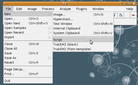
1. Getting startedOpen the Script Editor by choosing "File - New - Script". |
|
||||||
|
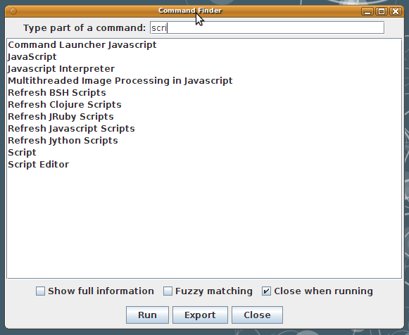
Alternatively, use the Command finder: Push 'l' (letter L) and then start typing "scri". You will see a list of Fiji commands, getting shorter the more letters you type. When the "Script Editor" command is visible, push the up arrow to go to it, and then push return to launch it. (Or double-click on it.) The Command Finder is useful for invoking any Fiji command. |
|
||||||
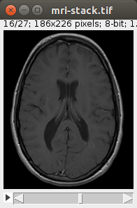
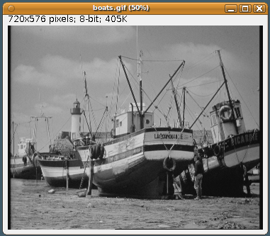
2. Your first Fiji scriptWe'll need an image to work on: please open any image. |
|
||||||
|
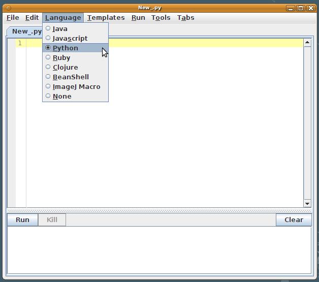
This tutorial will use the programming language Python 2.7. We start by telling the opened Script Editor what language you want to write the script on: choose "Language - Python". |
|
||||||
|
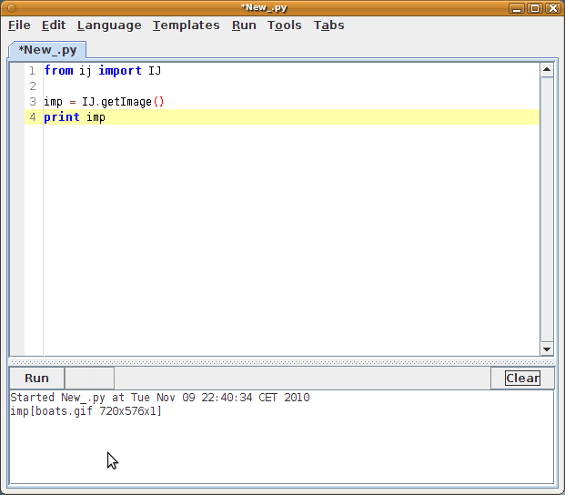
Type in what you see on the image to the right into the Script Editor, and then push "Run", or choose "Run - Run", or control+R (command+R in MacOSX). Line by line:
So what is "imp"? "imp" is a commonly used name to refer to an instance of an ImagePlus. The ImagePlus is one of ImageJ's abstractions to represent an image. Every image that you open in ImageJ is an instance of ImagePlus. |
|
||||||
|
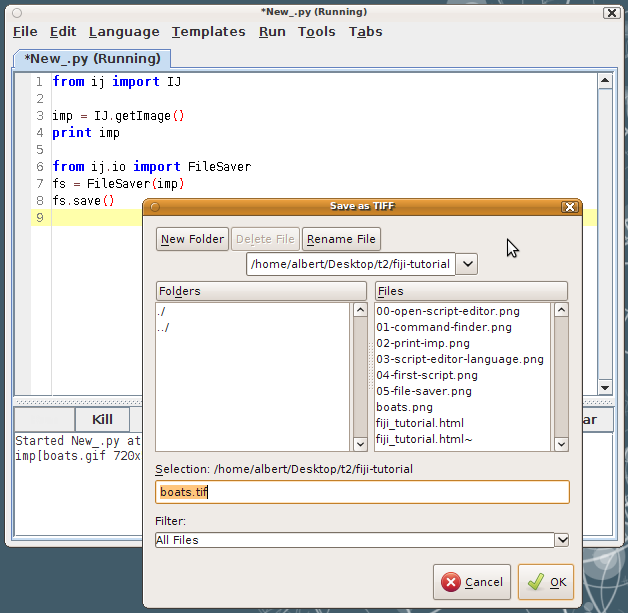
Saving an image with a file dialog The first action we'll do on our image is to save it. To do that, you could call "File - Save" from the menus. |
|
||||||
|
Saving an image directly to a file The point of running a script is to avoid human interaction. Notice that the '#' sign defines comments. In python, any text after a '#' is not executed. |
from ij import IJ
from ij.io import FileSaver

imp = IJ.getImage()
fs = FileSaver(imp)

# A known folder to store the image at:
folder = "/home/albert/Desktop/t2/fiji-tutorial"

filepath = folder + "/" + "boats.tif"
fs.saveAsTiff(filepath):
|
||||||
|
Saving an image ... checking first if it's a good idea. The FileSaver will overwrite whatever file exists at the file path that you give it. That is not always a good idea! Here, we write the same code but checking first:
And finally, if all expected preconditions hold, then we place the call to saveAsTiff. This script introduced three new programming items:
|
from ij import IJ
from ij.io import FileSaver
from os import path

imp = IJ.getImage()
fs = FileSaver(imp)

# A known folder to store the image at:
folder = "/home/albert/Desktop/t2/fiji-tutorial"

# Test if the folder exists before attempting to save the image:
if path.exists(folder) and path.isdir(folder):
  print "folder exists:", folder
  filepath = path.join(folder, "boats.tif") # Operating System-specific
  if path.exists(filepath):
    print "File exists! Not saving the image, would overwrite a file!"
  elif fs.saveAsTiff(filepath):
    print "File saved successfully at ", filepath
else:
  print "Folder does not exist or it's not a folder!"
|
||||||
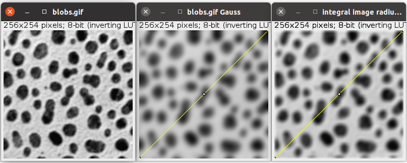
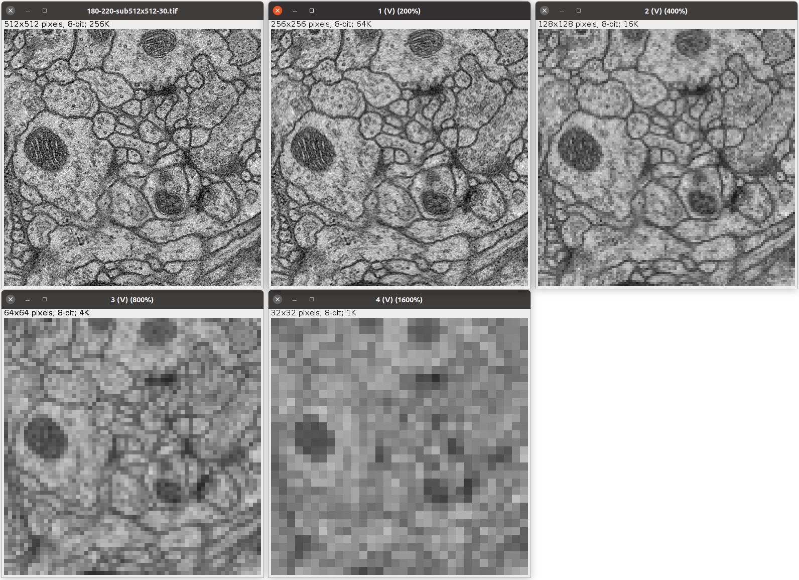
3. Inspecting properties and pixels of an imageAn image in ImageJ or Fiji is, internally, an instance of ImagePlus. In python, accessing fields of an instance is straightforward: just add a dot '.' between the variable "imp" and the field "title" to access. In the Fiji API documentation, if you don't see a specific field like width in a particular class, but there is a getWidth method, then from python they are one and the same. The image type Notice how we created a dictionary to hold key/value pairs: of the image type versus a text representation of that type. This dictionary (also called map or table in other programming languages) then lets us ask it for a specific image type (such as ImagePlus.GRAY8), and we get back the corresponding text, such as "8-bit". You may have realized by now that the ImagePlus.getType() (or what is the same in python: "imp.type") returns us any of the controled values of image type that an ImagePlus instance can take. These values are GRAY8, GRAY16, GRAY32, COLOR_RGB, and COLOR_256. What is the image type? It's the kind of pixel data that the image holds. It could be numbers from 0 to 255 (what fits in an 8-bit range), or from 0 to 65536 (values that fit in a 16-bit range), or could be three channels of 8-bit values (an RGB image), or floating-point values (32-bit). The COLOR_256 indicates an 8-bit image that has an associated look-up table: each pixel value does not represent an intensity, but rather it's associated with a color. The table of values versus colors is limited to 256, and hence these images may not look very well. For image processing, you should avoid COLOR_256 images (also known as "8-bit color" images). These images are meant for display in the web in ".gif" format, but have been superseeded by JPEG or PNG. The GRAY_8 ("8-bit"), GRAY_16 ("16-bit") and GRAY_32 ("32-bit") images may also be associated with a look-up table. For example, in a "green" look-up table on an 8-bit image, values of zero are black, values of 128 are darkish green, and the maximum value of 255 is fully pure green. |
from ij import IJ, ImagePlus

# Grab the last activated image
imp = IJ.getImage()

# Print image details
print "title:", imp.title
print "width:", imp.width
print "height:", imp.height
print "number of pixels:", imp.width * imp.height
print "number of slices:", imp.getNSlices()
print "number of channels:", imp.getNChannels()
print "number of time frames:", imp.getNFrames()

types = {ImagePlus.COLOR_RGB : "RGB",
         ImagePlus.GRAY8 : "8-bit",
         ImagePlus.GRAY16 : "16-bit",
         ImagePlus.GRAY32 : "32-bit",
         ImagePlus.COLOR_256 : "8-bit color"}

print "image type:", types[imp.type]
Started New_.py at Wed Nov 10 14:57:46 CET 2010
title: boats.gif
width: 720
height: 576
number of pixels: 414720
number of slices: 1
number of channels: 1
number of time frames: 1
image type: 8-bit
|
||||||
|
Obtaining pixel statistics of an image (and your first function) ImageJ / Fiji offers an ImageStatistics class that does all the work for us. Notice how we import the ImageStatistics namespace as "IS", i.e. we alias it--it's too long to type! The options variable is the bitwise-or combination of three different static fields of the ImageStatistics class. The final options is an integer that has specific bits set that indicate mean, median and min and max values. |
from ij import IJ
from ij.process import ImageStatistics as IS

# Grab the active image
imp = IJ.getImage()

# Get its ImageProcessor
ip = imp.getProcessor()

options = IS.MEAN | IS.MEDIAN | IS.MIN_MAX
stats = IS.getStatistics(ip, options, imp.getCalibration())

# print statistics on the image
print "Image statistics for", imp.title
print "Mean:", stats.mean
print "Median:", stats.median
print "Min and max:", stats.min, "-", stats.max
Started New_.py at Wed Nov 10 19:54:37 CET 2010
Image statistics for boats.gif
Mean: 120.026837384
Median: 138.0
Min and max: 3.0 - 220.0
|
||||||
|
Now, how about obtaining statistics for a lot of images? (in other words, batch processing).
So we define a folder that contains our images, and we loop the list of filenames that it has. For every filename that ends with ".tif", we load it as an ImagePlus, and handle it to the getStatistics function, which returns us the mean, median, and min and max values. (Note: if the images are stacks, use StackStatistics instead.) This script introduces a few new concepts:
See also the python documentation page on control flow, with explanations on the keywords if, else and elif, the for loop keyword and the break and continue keywords, defining a function with def, functions with variable number of arguments, anonymous functions (with the keyword lambda), and guidelines on coding style. |
from ij import IJ
from ij.process import ImageStatistics as IS
import os

options = IS.MEAN | IS.MEDIAN | IS.MIN_MAX

def getStatistics(imp):
  """ Return statistics for the given ImagePlus """
  ip = imp.getProcessor()
  stats = IS.getStatistics(ip, options, imp.getCalibration())
  return stats.mean, stats.median, stats.min, stats.max


# Folder to read all images from:
folder = "/home/albert/Desktop/t2/fiji-tutorial"

# Get statistics for each image in the folder
# whose file extension is ".tif":
for filename in os.listdir(folder):
  if filename.endswith(".tif"):
    print "Processing", filename
    imp = IJ.openImage(os.path.join(folder, filename))
    if imp is None:
      print "Could not open image from file:", filename
      continue
    mean, median, min, max = getStatistics(imp)
    print "Image statistics for", imp.title
    print "Mean:", mean
    print "Median:", median
    print "Min and max:", min, "-", max
  else:
    print "Ignoring", filename
|
||||||
|
Iterating pixels Iterating pixels is considered a low-level operation that you would seldom, if ever, have to do. But just so you can do it when you need to, here are various ways to iterate all pixels in an image. The three iteration methods:
The last should be your preferred method. There's the least opportunity for introducting an error, and it is very concise. Regarding the example given, keep in mind:
|
from ij import IJ
from sys.float_info import max as MAX_FLOAT

# Grab the active image
imp = IJ.getImage()

# Grab the image processor converted to float values
# to avoid problems with bytes
ip = imp.getProcessor().convertToFloat() # as a copy
# The pixels points to an array of floats
pixels = ip.getPixels()

print "Image is", imp.title, "of type", imp.type

# Obtain the minimum pixel value

# Method 1: the for loop, C style
minimum = MAX_FLOAT
for i in xrange(len(pixels)):
  if pixels[i] < minimum:
    minimum = pixels[i]

print "1. Minimum is:", minimum

# Method 2: iterate pixels as a list
minimum = MAX_FLOAT
for pix in pixels:
  if pix < minimum:
    minimum = pix

print "2. Minimum is:", minimum

# Method 3: apply the built-in min function
# to the first pair of pixels,
# and then to the result of that and the next pixel, etc.
minimum = reduce(min, pixels)

print "3. Minimum is:", minimum
Started New_.py at Wed Nov 10 20:49:31 CET 2010
Image is boats.gif of type 0
1. Minimum is: 3.0
2. Minimum is: 3.0
3. Minimum is: 3.0
|
||||||
|
On iterating or looping lists or collections of elements Ultimately all operations that involve iterating a list or a collection of elements can be done with the for looping construct. But in almost all occasions the for is not the best choice, neither regarding performance nor in clarity or conciseness. The latter is important to minimize the amount of errors that we may possibly introduce without noticing. There are three kinds of operations to perform on lists or collections: map, reduce, and filter. We show them here along with the equivalent for loop. |
|||||||
|
A map operation takes a list of length N and returns another list also of length N, with the results of applying a function (that takes a single argument) to every element of the original list. For example, suppose you want to get a list of all images open in Fiji. With the for loop, we have to create first a list explictly and then append one by one every image. With list comprehension, the list is created directly and the logic of what goes in it is placed inside the square brackets--but it is still a loop. That is, it is still a sequential, unparallelizable operation. With the map, we obtain the list automatically by executing the function WM.getImage to every ID in the list of IDs. While this is a trivial example, suppose you were executing a complex operation on every element of a list or an array. If you were to redefine the map function to work in parallel, suddenly any map operation in your program will run faster, without you having to modify a single line of tested code! |
from ij import WindowManager as WM

# Method 1: with a 'for' loop
images = []
for id in WM.getIDList():
  images.append(WM.getImage(id))

# Method 2: with list comprehension
images = [WM.getImage(id) for id in WM.getIDList()]

# Method 3: with a 'map' operation
images = map(WM.getImage, WM.getIDList())
|
||||||
|
A filter operation takes a list of length N and returns a shorter list, with anywhere from 0 to N elements. Only those elements of the original list that pass a test are placed in the new, returned list. For example, suppose you want to find the subset of opened images in Fiji whose title match a specific criterium. With the for loop, we have to create a new list first, and then append elements to that list as we iterate the list of images. The second variant of the for loop uses list comprehension. The code is reduced to a single short line, which is readable, but is still a python loop (with potentially lower performance). With the filter operation, we get the (potentially) shorter list automatically. The code is a single short line, instead of 4 lines! |
from ij import WindowManager as WM

# A list of all open images
imps = map(WM.getImage, WM.getIDList())

def match(imp):
  """ Returns true if the image title contains the word 'cochlea'"""
  return imp.title.find("cochlea") > -1

# Method 1: with a 'for' loop
# (We have to explicitly create a new list)
matching = []
for imp in imps:
  if match(imp):
    matching.append(imp)

# Method 2: with list comprehension
matching = [imp for imp in imps if match(imp)]

# Method 3: with a 'filter' operation
matching = filter(match, imps)
|
||||||
|
A reduce operation takes a list of length N and returns a single value. This value is composed from applying a function that takes two arguments to the first two elements of the list, then to the result of that and the next element, etc. Optionally an initial value may be provided, so that the cycle starts with that value and the first element of the list. For example, suppose you want to find the largest image, by area, from the list of all opened images in Fiji. With the for loop, we have to we have to keep track of which was the largest area in a pair of temporary variables. And even check whether the stored largest image is null! We could have initizalized the largestArea variable to the first element of the list, and then start looping at the second element by slicing the first element off the list (with "for imp in imps[1:]:"), but then we would have had to check if the list contains at least one element. With the reduce operation, we don't need any temporary variables. All we need is to define a helper function (which could have been an anonymous lambda function, but we defined it explicitly for extra clarity and reusability). |
from ij import IJ

from ij import WindowManager as WM

# A list of all open images
imps = map(WM.getImage, WM.getIDList())

def area(imp):
  return imp.width * imp.height

# Method 1: with a 'for' loop
largest = None
largestArea = 0
for imp in imps:
  a = area(imp)
  if largest is None:
    largest = imp
    largestArea = a
  else:
    if a > largestArea:
      largest = imp
      largestArea = a

# Method 2: with a 'reduce' operation
def largestImage(imp1, imp2):
  return imp1 if area(imp1) > area(imp2) else imp2

largest = reduce(largestImage, imps)
|
||||||
|
Subtract the min value to every pixel First we obtain the minimum pixel value, using the reduce method explained just above. Then we subtract this minimum value to every pixel. We have two ways to do it:
With the first method, since the pixels array was already a copy (notice we called convertToFloat() on the ImageProcessor), we can use it to create a new ImagePlus with it without any unintended consequences. With the second method, the new list of pixels must be given to a new FloatProcessor instance, and with it, a new ImagePlus is created, of the same dimensions as the original. |
from ij import IJ, ImagePlus
from ij.process import FloatProcessor

imp = IJ.getImage()
ip = imp.getProcessor().convertToFloat() # as a copy
pixels = ip.getPixels()

# Apply the built-in min function
# to the first pair of pixels,
# and then to the result of that and the next pixel, etc.
minimum = reduce(min, pixels)

# Method 1: subtract the minim from every pixel,
# in place, modifying the pixels array
for i in xrange(len(pixels)):
  pixels[i] -= minimum
# ... and create a new image:
imp2 = ImagePlus(imp.title, ip)

# Method 2: subtract the minimum from every pixel
# and store the result in a new array
pixels3 = map(lambda x: x - minimum, pixels)
# ... and create a new image:
ip3 = FloatProcessor(ip.width, ip.height, pixels3, None)
imp3 = ImagePlus(imp.title, ip3)

# Show the images in an ImageWindow:
imp2.show()
imp3.show()
|
||||||
|
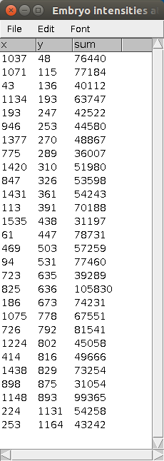
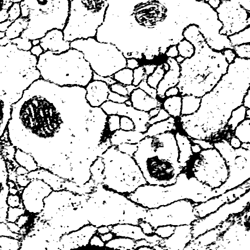
Reduce a pixel array to a single value: count pixels above a threshold Suppose you want to analyze a subset of pixels. For example, find out how many pixels have a value over a certain threshold. The reduce built-in function is made just for that. It takes a function with two arguments (the running count and the next pixel); the list or array of pixels; and an initial value (in this case, zero) for the first argument (the "count'), and will return a single value (the total count). In this example, we computed first the mean pixel intensity, and then filtered all pixels for those whose value is above the mean. Notice that we compute the mean by using the convenient built-in function sum, which is able to add all numbers contained in any kind of collection (be it a list, a native array, a set of unique elements, or the keys of a dictionary). We could imitate the built-in sum function with reduce(lambda s, x: s + x, pixels), but paying a price in performance. Notice we are using anonymous functions again (that is, functions that lack a name), declared in place with the lambda keyword. A function defined with def would do just fine as well. |
from ij import IJ

# Grab currently active image
imp = IJ.getImage()
ip = imp.getProcessor().convertToFloat()
pixels = ip.getPixels()

# Compute the mean value (sum of all divided by number of pixels)
mean = sum(pixels) / len(pixels)

# Count the number of pixels above the mean
n_pix_above = reduce(lambda count, a: count + 1 if a > mean else count, pixels, 0)

print "Mean value", mean
print "% pixels above mean:", n_pix_above / float(len(pixels)) * 100
Started New_.py at Thu Nov 11 01:50:49 CET 2010
Mean value 120.233899981
% pixels above mean: 66.4093846451
|
||||||
|
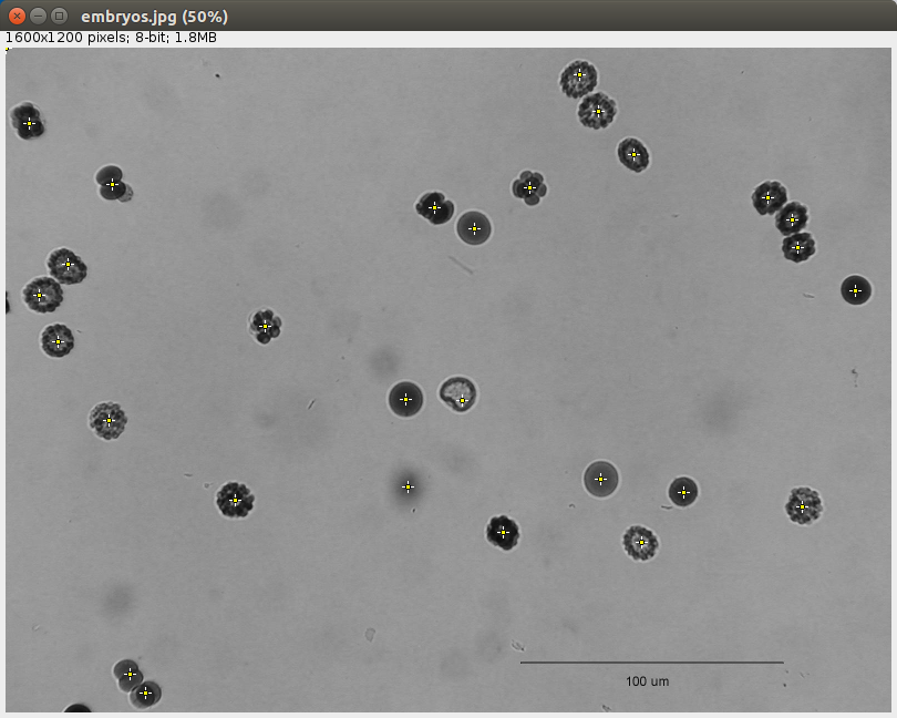
Another useful application of filtering pixels by their value: finding the coordinates of all pixels above a certain value (in this case, the mean), and then calculating their center of mass. The filter built-in function is made just for that. The indices of the pixels whose value is above the mean are collected in a list named "above", which is created by filtering the indices of all pixels (provided by the built-in function xrange). The filtering is done by an anonymous function declared with lambda, with a single argument: the index i of the pixel. Here, note that in ImageJ, the pixels of an image are stored in a linear array. The length of the array is width * height, and the pixels are stored as concatenated rows. Therefore, the modulus of dividing the index of a pixel by the width the image provides the X coordinate of a pixel. Similarly, the integer division of the index of a pixel by the width provides the Y coordinate. To compute the center of mass, there are two equivalent methods. The C-style method with a for loop, with every variable being declared prior to the loop, and then modified at each loop iteration and, after the loop, dividing the sum of coordinates by the number of coordinates (the length of the "above" list). For this example, this is the method with the best performance.The second method computes the X and Y coordinates of the center of mass with a single line of code for each. Notice that both lines are nearly identical, differing only in the body of the function mapped to the "above" list containing the indices of the pixels whose value is above the mean. While, in this case, the method is less performant due to repeated iteration of the list "above", the code is shorter, easier to read, and with far less opportunities for introducing errors. If the actual computation was far more expensive than the simple calculation of the coordinates of a pixel given its index in the array of pixels, this method would pay off for its clarity. |
from ij import IJ

# Grab the currently active image
imp = IJ.getImage()
ip = imp.getProcessor().convertToFloat()
pixels = ip.getPixels()

# Compute the mean value
mean = sum(pixels) / len(pixels)

# Obtain the list of indices of pixels whose value is above the mean
above = filter(lambda i: pixels[i] > mean, xrange(len(pixels)))

print "Number of pixels above mean value:", len(above)

# Measure the center of mass of all pixels above the mean

# The width of the image, necessary for computing the x,y coordinate of each pixel
width = imp.width

# Method 1: with a for loop
xc = 0
yc = 0
for i in above:
  xc += i % width # the X coordinate of pixel at index i
  yc += i / width # the Y coordinate of pixel at index i
xc = xc / len(above)
yc = yc / len(above)
print xc, yc

# Method 2: with sum and map
xc = sum(map(lambda i: i % width, above)) / len(above)
yc = sum(map(lambda i: i / width, above)) / len(above)
print xc, yc
|
||||||
|
The third method pushes the functional approach too far. While written in a single line, that doesn't mean it is clearer to read: it's intent is obfuscated by starting from the end: the list comprehension starts off by stating that each element (there are only two) of the list resulting from the reduce has to be divided by the length of the list of pixels "above", and only then we learn than the collection being iterated is the array of two coordinates, created at every iteration over the list "above", containing the sum of all coordinates for X and for Y. Notice that the reduce is invoked with three arguments, the third one being the list [0, 0] containing the initialization values of the sums. Confusing! Avoid writing code like this. Notice as well that, by creating a new list at every iteration step, this method is the least performant of all. The fourth method is a clean up of the third method. Notice that we import the partial function from the functools package. With it, we are able to create a version of the "accum" helper function that has a frozen "width" argument (also known as currying a function). In this way, the "accum" function is seen by the reduce as a two-argument function (which is what reduce needs here). While we regain the performance of the for loop, notice that now the code is just as long as with the for loop. The purpose of writing this example is to illustrate how one can write python code that doesn't use temporary variables, these generally being potential points of error in a computer program. It is always better to write lots of small functions that are easy to read, easy to test, free of side effects, documented, and that then can be used to assemble our program. |
# (Continues from above...)

# Method 3: iterating the list "above" just once
xc, yc = [d / len(above) for d in
            reduce(lambda c, i: [c[0] + i % width, c[1] + i / width], above, [0, 0])]
print xc, yc

# Method 4: iterating the list "above" just once, more clearly and performant
from functools import partial

def accum(width, c, i):
  """ Accumulate the sum of the X,Y coordinates of index i in the list c."""
  c[0] += i % width
  c[1] += i / width
  return c

xy, yc = [d / len(above) for d in reduce(partial(accum, width), above, [0, 0])]
print xc, yc
|
||||||
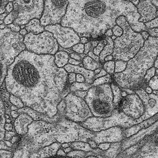
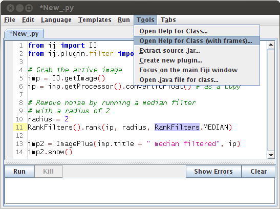
4. Running ImageJ / Fiji plugins on an ImagePlusHere is an example plugin run programmatically: a median filter applied to the currently active image. The median filter, along with the mean, minimum, maximum, variance, remove outliers and despeckle menu commands, are implemented in the RankFilters class. |
from ij import IJ, ImagePlus
from ij.plugin.filter import RankFilters

# Grab the active image
imp = IJ.getImage()
ip = imp.getProcessor().convertToFloat() # as a copy

# Remove noise by running a median filter
# with a radius of 2
radius = 2
RankFilters().rank(ip, radius, RankFilters.MEDIAN)

imp2 = ImagePlus(imp.title + " median filtered", ip)
imp2.show()
|
||||||
|
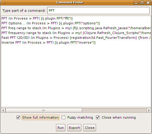
Finding the class that implements a specific ImageJ command When starting ImageJ/Fiji programming, the problem is not so much how to run a plugin on an image, as it is to find out which class implements which plugin. Here is a simple method to find out, via the Command Finder:
Notice that the plugin class comes with some text. For example:
FFT (in Process > FFT) [ij.plugin.FFT("fft")]
Inverse FFT (in Process > FFT) [ij.plugin.FFT("inverse")]
The above two commands are implemented by a single plugin (ij.plugin.FFT) whose run method accepts, like all PlugIn, a text string specifying the action: the fft, or the inverse. |
|
||||||
|
Finding the java documentation for any class Once you have found the PlugIn class that implements a specific command, you may want to use that class directly. The information is either in the online java documentation or in the source code. How to find these?
|
|
||||||
|
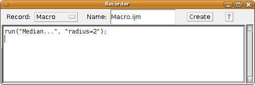
Figuring out what parameters a plugin requires To do that, we'll use the Macro Recorder. Make sure that an image is open. Then:
That is valid macro code, that ImageJ can execute. The first part is the command ("Median..."), the second part is the parameters that that command uses; in this case, just one ("radius=2"). If there were more parameters, they would be separated by spaces. Note that boolean parameters are true (the checkbox in the dialog is ticked) when present at all in the list of parameters of the macro code, and false otherwise (by default). |
|
||||||
|
Running a command on an image We can use these macro recordings to create jython code that executes a given plugin on a given image. Here is an example. Very simple! The IJ namespace has a function, run, that accepts an ImagePlus as first argument, then the name of the command to run, and then the macro-ready list of arguments that the command requires. |
from ij import IJ

# Grab the active image
imp = IJ.getImage()

# Run the median filter on it, with a radius of 2
IJ.run(imp, "Median...", "radius=2")
|
||||||
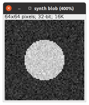
5. Creating images and regions of interest (ROIs)Create an image from scratch An ImageJ/Fiji image is composed of at least three objects:
In the example, we create an empty array of floats (see creating native arrays), and fill it in with random float values. Then we give it to a FloatProcessor instance, which is then wrapped by an ImagePlus instance. Voilà! |
from ij import ImagePlus
from ij.process import FloatProcessor
from array import zeros
from random import random

width = 1024
height = 1024
pixels = zeros('f', width * height)

for i in xrange(len(pixels)):
  pixels[i] = random()

fp = FloatProcessor(width, height, pixels, None)
imp = ImagePlus("White noise", fp)

imp.show()
|
||||||
|
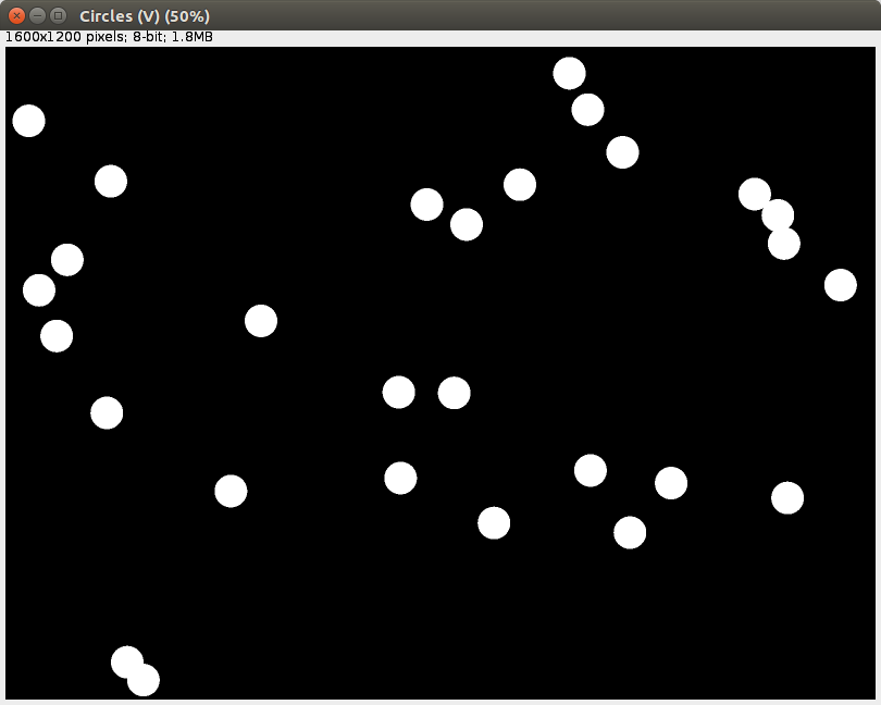
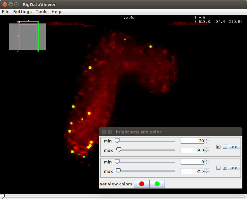
Fill a region of interest (ROI) with a given value To fill a region of interest in an image, we could iterate the pixels, find the pixels that lay within the bounds of interest, and set their values to a specified value. But that tedious and error prone. Much more effective is to create an instance of a Roi class or one of its subclasses (PolygonRoi, OvalRoi, ShapeRoi, etc.) and tell the ImageProcessor to fill that region. In this example, we create an image filled with white noise like before, and then define a rectangular region of interest in it, which is filled with a value of 2.0. The white noise is drawn from a random distribution whose values range from 0 to 1. When filling an area of the FloatProcessor with a value of 2.0, that is the new maximum value. The area with 2.0 pixel values will look white (look at the status bar): 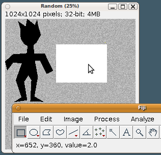
|
from ij import IJ, ImagePlus
from ij.process import FloatProcessor
from array import zeros
from random import random
from ij.gui import Roi, PolygonRoi

# Create a new ImagePlus filled with noise
width = 1024
height = 1024
pixels = zeros('f', width * height)

for i in xrange(len(pixels)):
  pixels[i] = random()

fp = FloatProcessor(width, height, pixels, None)
imp = ImagePlus("Random", fp)

# Fill a rectangular region of interest
# with a value of 2:
roi = Roi(400, 200, 400, 300)
fp.setRoi(roi)
fp.setValue(2.0)
fp.fill()

# Fill a polygonal region of interest
# with a value of -3
xs = [234, 174, 162, 102, 120, 123, 153, 177, 171,
      60, 0, 18, 63, 132, 84, 129, 69, 174, 150,
      183, 207, 198, 303, 231, 258, 234, 276, 327,
      378, 312, 228, 225, 246, 282, 261, 252]
ys = [48, 0, 60, 18, 78, 156, 201, 213, 270, 279,
      336, 405, 345, 348, 483, 615, 654, 639, 495,
      444, 480, 648, 651, 609, 456, 327, 330, 432,
      408, 273, 273, 204, 189, 126, 57, 6]
proi = PolygonRoi(xs, ys, len(xs), Roi.POLYGON)
fp.setRoi(proi)
fp.setValue(-3)
fp.fill(proi.getMask())  # Attention!

imp.show()
|
||||||
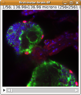
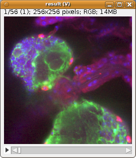
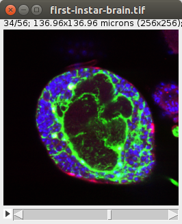
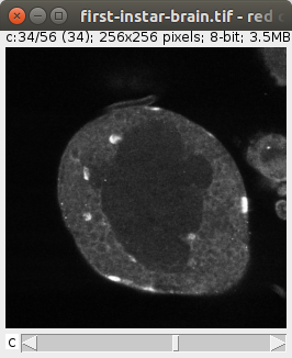
6. Create and manipulate image stacks and hyperstacksLoad a color image stack and extract its green channel First we load the stack from the web--it's the "Fly Brain" sample image. Then we iterate its slices. Each slice is a ColorProcessor: wraps an integer array. Each integer is represented by 4 bytes, and the lower 3 bytes represent, respectively, the intensity values for red, green and blue. The upper most byte is usually reserved for alpha (the inverse of transparency), but ImageJ ignores it. Dealing with low-level details like that is not necessary. The ColorProcessor has a method, toFloat, that can give us a FloatProcessor for a specific color channel. Red is 0, green is 1, and blue is 2. Representing the color channel in floats is most convenient for further processing of the pixel values--won't overflow like a byte would. In this example, all we do is collect each slice into a list of slices we named greens. Then we add all the slices to a new ImageStack, and pass it to a new ImagePlus. Then we invoke the "Green" command on that ImagePlus instance, so that a linear green look-up table is assigned to it. And we show it. |
from ij import IJ, ImagePlus, ImageStack

# Load a stack of images: a fly brain, in RGB
imp = IJ.openImage("https://imagej.nih.gov/ij/images/flybrain.zip")
stack = imp.getImageStack()

print "number of slices:", imp.getNSlices()

# A list of green slices
greens = []

# Iterate each slice in the stack
for i in xrange(1, imp.getNSlices()+1):
  # Get the ColorProcessor slice at index i
  cp = stack.getProcessor(i)
  # Get its green channel as a FloatProcessor
  fp = cp.toFloat(1, None)
  # ... and store it in a list
  greens.append(fp)

# Create a new stack with only the green channel
stack2 = ImageStack(imp.width, imp.height)
for fp in greens:
  stack2.addSlice(None, fp)

# Create a new image with the stack of green channel slices
imp2 = ImagePlus("Green channel", stack2)
# Set a green look-up table:
IJ.run(imp2, "Green", "")
imp2.show()
|
||||||
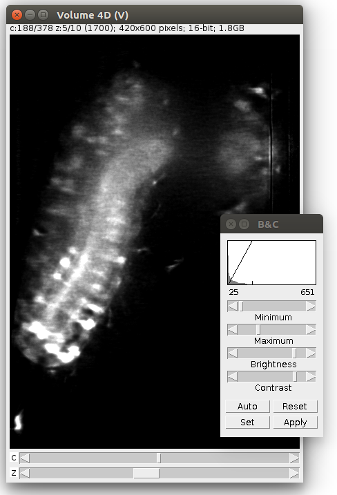
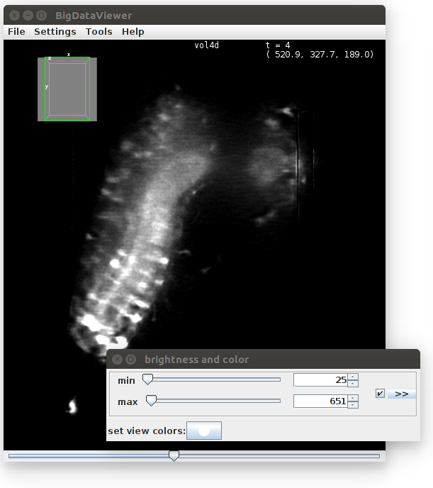
|
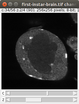
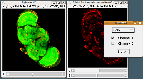
Convert an RGB stack to a 2-channel, 32-bit hyperstack We load an RGB stack--the "Fly brain" sample image, as before. Suppose we want to analyze each color channel independently: an RGB image doesn't really let us, without lots of low-level work to disentangle the different color values from each pixel value. So we convert the RGB stack to a hyperstack with two separate channels, where each channel slice is a 32-bit FloatProcessor. The first step is to create a new ImageStack instance, to hold all the slices that we'll need: one per color channel, times the number of slices. Realize that we could have 7 channels if we wanted, or 20, for each slice. As many as you want. The final step is to open the hyperstack. For that:
Open the "Image - Color - Channels Tool" and you'll see that the Composite image is set to show only the red channel--try checking the second channel as well. For a real-world example of a python script that uses hyperstacks, see the Correct_3D_drift.py script (available as the command "Plugins - Registration - Correct 3D drift"). |
from ij import IJ, ImagePlus, ImageStack, CompositeImage

# Load a stack of images: a fly brain, in RGB
imp = IJ.openImage("https://imagej.nih.gov/ij/images/flybrain.zip")
stack = imp.getImageStack()

# A new stack to hold the data of the hyperstack
stack2 = ImageStack(imp.width, imp.height)

# Convert each color slice in the stack
# to two 32-bit FloatProcessor slices
for i in xrange(1, imp.getNSlices()+1):
  # Get the ColorProcessor slice at index i
  cp = stack.getProcessor(i)
  # Extract the red and green channels as FloatProcessor
  red = cp.toFloat(0, None)
  green = cp.toFloat(1, None)
  # Add both to the new stack
  stack2.addSlice(None, red)
  stack2.addSlice(None, green)

# Create a new ImagePlus with the new stack
imp2 = ImagePlus("32-bit 2-channel composite", stack2)
imp2.setCalibration(imp.getCalibration().copy())

# Tell the ImagePlus to represent the slices in its stack
# in hyperstack form, and open it as a CompositeImage:
nChannels = 2             # two color channels
nSlices = stack.getSize() # the number of slices of the original stack
nFrames = 1               # only one time point
imp2.setDimensions(nChannels, nSlices, nFrames)
comp = CompositeImage(imp2, CompositeImage.COLOR)
comp.show()
|
||||||
7. Interacting with humans: file and option dialogs, messages, progress bars.Ask the user for a directory See DirectoryChooser. |
from ij.io import DirectoryChooser

dc = DirectoryChooser("Choose a folder")
folder = dc.getDirectory()

if folder is None:
  print "User canceled the dialog!"
else:
  print "Selected folder:", folder
|
||||||
|
Ask the user for a file See OpenDialog and SaveDialog. |
from ij.io import OpenDialog

od = OpenDialog("Choose a file", None)
filename = od.getFileName()

if filename is None:
  print "User canceled the dialog!"
else:
  directory = od.getDirectory()
  filepath = directory + filename
  print "Selected file path:", filepath
|
||||||
|
Show a progress bar Will show a progress bar in the Fiji window. |
from ij import IJ

imp = IJ.getImage()
stack = imp.getImageStack()

for i in xrange(1, stack.getSize()+1):
  # Report progress
  IJ.showProgress(i, stack.getSize()+1)
  # Do some processing
  ip = stack.getProcessor(i)
  # ...

# Signal completion
IJ.showProgress(1)
|
||||||
|
Ask the user to enter a few parameters in a dialog There are more possibilities, but these are the basics. See GenericDialog. All plugins that use a GenericDialog are automatable. Remember how above we run a command on an image? When the names in the dialog fields match the names in the macro string, the dialog is fed in the values automatically. If a dialog field doesn't have a match, it takes the default value as defined in the dialog declaration. If a plugin was using a dialog like the one we built here, we would run it automatically like this:
args = "name='first' alpha=0.5 output='32-bit' scale=80"

IJ.run(imp, "Some PlugIn", args)
Above, leaving out the word 'optimize' means that it will use the default value (True) for it. |
from ij.gui import GenericDialog

def getOptions():
  gd = GenericDialog("Options")
  gd.addStringField("name", "Untitled")
  gd.addNumericField("alpha", 0.25, 2)  # show 2 decimals
  gd.addCheckbox("optimize", True)
  types = ["8-bit", "16-bit", "32-bit"]
  gd.addChoice("output as", types, types[2])
  gd.addSlider("scale", 1, 100, 100)
  gd.showDialog()
  #
  if gd.wasCanceled():
    print "User canceled dialog!"
    return
  # Read out the options
  name = gd.getNextString()
  alpha = gd.getNextNumber()
  optimize = gd.getNextBoolean()
  output = gd.getNextChoice()
  scale = gd.getNextNumber()
  return name, alpha, optimize, output, scale # a tuple with the parameters

options = getOptions()
if options is not None:
  name, alpha, optimize, output, scale = options # unpack each parameter
  print name, alpha, optimize, output, scale
|
||||||
|
A reactive dialog: using a preview checkbox Now that you know how to use ImageJ's GenericDialog, here we show how to implement the functionality of a preview checkbox. A preview checkbox is present in many plugins that use a GenericDialog for its options. Instead of waiting for the user to push the "OK" button, the image is updated dynamically, in response to user input--that is, to the user entering a numeric value into a text field, or, in this example, moving a Scrollbar. The key concept is that of a listener. All user interface (UI) elements allow us to register our own functions so that, when there is an update (e.g. the user pushes a keystroke while the UI element is activated, or the mouse is moved or clicked), our function is executed, giving us the opportunity to react to user input. Each type of UI element has its own type of listener. The Scrollbar used here allows us to register an AdjustmentListener. We implement this interface with our class ScalingPreviewer and its method adjustmentValueChanged. Given that the scrollbar can generate many events as the user drags its handle with the mouse, we are only interested in the last event, and therefore we check for event.getValueIsAdjusting() which tells us, when returning True, that by the time we are processing this event there are already more events queued, and then we terminate execution of our response with return. The next event in the queue will ask this question again, and only the last event will proceed to execute self.scale(). When the user again clicks to drag the scroll bar handle, all of this starts again. If the preview checkbox is not ticked, our listener doesn't do anything. If the preview box was not ticked, and then it is, our ScalingPreviewer, which also implements ItemListener (with its only method itemStateChanged) is also registered as a listener for the checkbox and responds, when the checkbox is selected, by calling self.scale(). When the user pushes "OK", the scaling is applied (even if it was already before; more logic would be needed to avoid this duplication when the preview checkbox is ticked). When cancelled, the original image is restored. |
# A reactive generic dialog

from ij.gui import GenericDialog
from ij import WindowManager as WM
from java.awt.event import AdjustmentListener, ItemListener

class ScalingPreviewer(AdjustmentListener, ItemListener):
  def __init__(self, imp, slider, preview_checkbox):
    """
       imp: an ImagePlus
       slider: a java.awt.Scrollbar UI element
       preview_checkbox: a java.awt.Checkbox controlling whether to
                         dynamically update the ImagePlus as the
                         scrollbar is updated, or not.
    """
    self.imp = imp
    self.original_ip = imp.getProcessor().duplicate() # store a copy
    self.slider = slider
    self.preview_checkbox = preview_checkbox

  def adjustmentValueChanged(self, event):
    """ event: an AdjustmentEvent with data on the state of the scroll bar. """
    preview = self.preview_checkbox.getState()
    if preview:
      if event.getValueIsAdjusting():
        return # there are more scrollbar adjustment events queued already
      print "Scaling to", event.getValue() / 100.0

      self.scale()

  def itemStateChanged(self, event):
    """ event: an ItemEvent with data on what happened to the checkbox. """
    if event.getStateChange() == event.SELECTED:
      self.scale()

  def reset(self):
    """ Restore the original ImageProcessor """
    self.imp.setProcessor(self.original_ip)

  def scale(self):
    """ Execute the in-place scaling of the ImagePlus. """
    scale = self.slider.getValue() / 100.0
    new_width = int(self.original_ip.getWidth() * scale)
    new_ip = self.original_ip.resize(new_width)
    self.imp.setProcessor(new_ip)


def scaleImageUI():
  gd = GenericDialog("Scale")
  gd.addSlider("Scale", 1, 200, 100)
  gd.addCheckbox("Preview", True)
  # The UI elements for the above two inputs
  slider = gd.getSliders().get(0) # the only one
  checkbox = gd.getCheckboxes().get(0) # the only one

  imp = WM.getCurrentImage()
  if not imp:
    print "Open an image first!"
    return

  previewer = ScalingPreviewer(imp, slider, checkbox)
  slider.addAdjustmentListener(previewer)
  checkbox.addItemListener(previewer)

  gd.showDialog()

  if gd.wasCanceled():
    previewer.reset()
    print "User canceled dialog!"
  else:
    previewer.scale()

scaleImageUI()
|
||||||
|
Managing UI-launched background tasks In the example above, the task to scale an image is run just like that: as soon as the UI element (the Scrollbar) notifies us--via our registered listener--, our listener function adjustmentValueChanged executes the task there and then. By doing so, the task is executed by the event dispatch thread: the same execution thread that updates the rendering of UI elements, and that processes any and all events emited from any UI element. In the case of the scaling task, it executes within milliseconds and we don't notice a thing. A task that would consume several seconds would make us realize that the UI has become unresponsive: clicking anywhere, or typing keys, would not result in any response--until our long-running task completes and then all queued events are executed, one at a time. Execution within the event dispatch thread is undesirable. Therefore, we must execute our task in a different thread. One option could be to submit our task to a thread pool that executes them as they come--but, for our example above, this would be undesirable: once we move the scrollbar, we don't care about prior positions (prior scaling values) the scrollbar held so far, and those tasks, if not yet completed, should be interrupted or not even started. A good solution is to delegate the execution to a ScheduledExecutorService, conveniently launched from Executors.newSingleThreadScheduledExecutor. This function creates a thread that periodically wakes up at fixed time intervals and then executes the function that we gave it--in this case, the ScalingPreviewer itself now implements the Runnable interface, and its only specified method, run, does the work: checks if there's anything to do relative to the last time it run, and if there is, executes it (so we pass self to scheduleWithFixedDelay, plus the timing arguments). This setup doesn't interrupt an update already in progress, but guarantees that we are always only executing one update at a time, and the latest update gets done the last--which is what matters. With this setup, the role of the adjustmentValueChanged is merely to change the state, that is, to update the state of requested_scaling_factor, which takes a negligible amount of time, therefore not interfering with the event dispatch thread's other tasks--and with the whole Fiji UI remaining responsive. Updating the state (the variables stored in the self.state dictionary) is done under a synchronization block: when a thread is accessing either getState or putState, no other thread can access either method, thanks to the function decorator make_synchronized (see below in the tutorial) that guarantees so (it's like java's synchronized reserved word). In principle we could have the self.state keys as member fields of the ScalingPreviewer class (i.e. self.requested_scaling_factor instead of the latter being a key of self.state), because updating a variable to a native value (a number, or a boolean) is an atomic operation. In Jython, though, it may not be--everything is an object, even numbers--and therefore it is best to access the state variables via synchronized methods, so that only one of the two threads does so at a time. It's also a good practice to access shared state under synchronization blocks, and this is a simple example illustrating how to do so. Notice near the end of the run method: the setProcessor is invoked via SwingUtilities.invokeAndWait method, using a lambda function (an anonymous function, which works here because all Jython functions implement the Runnable interface, required by invokeAndWait). This indirection is necessary because setProcessor will resize the window showing the image, and any operation that updates the UI must be run within the event dispatch thread to avoid problems. So yes: different methods of the ScalingPreviewer class are executed by different threads, and that's exactly the desirable setup. Once the user pushes the "OK" or "Cancel" buttons, we must invoke destroy(). Otherwise, the scheduled executor would keep running until quitting Fiji. The destroy() method requests its shutdown(), which will happen when the scheduled executor runs one more, and last, time.
|
# A reactive generic dialog that updates previews in the background

from ij.gui import GenericDialog
from ij import WindowManager as WM
from java.awt.event import AdjustmentListener, ItemListener
from java.util.concurrent import Executors, TimeUnit
from java.lang import Runnable
from javax.swing import SwingUtilities
from synchronize import make_synchronized

class ScalingPreviewer(AdjustmentListener, ItemListener, Runnable):
  def __init__(self, imp, slider, preview_checkbox):
    """
       imp: an ImagePlus
       slider: a java.awt.Scrollbar UI element
       preview_checkbox: a java.awt.Checkbox controlling whether to
                         dynamically update the ImagePlus as the
                         scrollbar is updated, or not.
    """
    self.imp = imp
    self.original_ip = imp.getProcessor().duplicate() # store a copy
    self.slider = slider
    self.preview_checkbox = preview_checkbox
    # Scheduled preview update
    self.scheduled_executor = Executors.newSingleThreadScheduledExecutor()
    # Stored state
    self.state = {
      "restore": False, # whether to reset to the original
      "requested_scaling_factor": 1.0, # last submitted request
      "last_scaling_factor": 1.0, # last executed request
      "shutdown": False, # to request terminating the scheduled execution
    }
    # Update, if necessary, every 300 milliseconds
    time_offset_to_start = 1000 # one second
    time_between_runs = 300
    self.scheduled_executor.scheduleWithFixedDelay(self,
      time_offset_to_start, time_between_runs, TimeUnit.MILLISECONDS)

  @make_synchronized
  def getState(self, *keys):
    """ Synchronized access to one or more keys.
        Returns a single value when given a single key,
        or a tuple of values when given multiple keys. """
    if 1 == len(keys):
      return self.state[keys[0]]
    return tuple(self.state[key] for key in keys)

  @make_synchronized
  def putState(self, key, value):
    self.state[key] = value

  def adjustmentValueChanged(self, event):
    """ event: an AdjustmentEvent with data on the state of the scroll bar. """
    preview = self.preview_checkbox.getState()
    if preview:
      if event.getValueIsAdjusting():
        return # there are more scrollbar adjustment events queued already
      self.scale()

  def itemStateChanged(self, event):
    """ event: an ItemEvent with data on what happened to the checkbox. """
    if event.getStateChange() == event.SELECTED:
      self.scale()

  def reset(self):
    """ Restore the original ImageProcessor """
    self.putState("restore", True)

  def scale(self):
    self.putState("requested_scaling_factor", self.slider.getValue() / 100.0)

  def run(self):
    """ Execute the in-place scaling of the ImagePlus,
        here playing the role of a costly operation. """
    if self.getState("restore"):
      print "Restoring original"
      ip = self.original_ip
      self.putState("restore", False)
    else:
      requested, last = self.getState("requested_scaling_factor", "last_scaling_factor")
      if requested == last:
        return # nothing to do
      print "Scaling to", requested
      new_width = int(self.original_ip.getWidth() * requested)
      ip = self.original_ip.resize(new_width)
      self.putState("last_scaling_factor", requested)

    # Request updating the ImageProcessor in the event dispatch thread,
    # given that the "setProcessor" method call will trigger
    # a change in the dimensions of the image window
    SwingUtilities.invokeAndWait(lambda: self.imp.setProcessor(ip))

    # Terminate recurrent execution if so requested
    if self.getState("shutdown"):
      self.scheduled_executor.shutdown()

  def destroy(self):
    self.putState("shutdown", True)

def scaleImageUI():
  gd = GenericDialog("Scale")
  gd.addSlider("Scale", 1, 200, 100)
  gd.addCheckbox("Preview", True)
  # The UI elements for the above two inputs
  slider = gd.getSliders().get(0) # the only one
  checkbox = gd.getCheckboxes().get(0) # the only one

  imp = WM.getCurrentImage()
  if not imp:
    print "Open an image first!"
    return

  previewer = ScalingPreviewer(imp, slider, checkbox)
  slider.addAdjustmentListener(previewer)
  checkbox.addItemListener(previewer)

  gd.showDialog()

  if gd.wasCanceled():
    previewer.reset()
    print "User canceled dialog!"
  else:
    previewer.scale()

  previewer.destroy()

scaleImageUI()
|
||||||
|
Building user interfaces (UI): basic concepts In addition to using ImageJ/Fiji's built-in methods for creating user interfaces, java offers a large and rich library to make your own custom user interfaces. Here, I explain how to create a new window and populate it with buttons, text fields and text labels, and how to use them. A basic example: create a window with a single button in it, that says "Measure", and which runs the "Analyze - Measure" command, first checking whether any image is open. First we declare the measure function, which checks whether an image is open, and if so, runs the measuring command like you learned above. Then we create a JFrame, which is the window itself with the typical buttons for closing or minimizing it. Note we give the constructor the keyword argument "visible": this is jython's way of short-circuiting a lot of boiler plate code that would be required in java. When invoking a constructor, in jython, you can take any public method whose name starts with "set", such as "setVisible" in JFrame, and instead invoke it by using "visible" (with lowercase first letter) as a keyword argument in the constructor. This is the so-called bean property architecture of get and set methods, e.g. if a class has a "setValue" (with one argument) and "getValue" (without arguments, returning the value) methods, use "value" directly as a keyword argument in the constructor, or as a public field like frame.visible = True, which is the exact same as frame.setVisible(True). When the button is instantiated, we also pass a method to its constructor as a keyword argument: actionPerformed=measure. While the mechanism is similar to the bean property system above, it is not the same: jython searches the listener interfaces that the class methods can accept for registration. In this case, the JButton class provides a method (addActionListener) that accepts as argument an object implementing the ActionListener interface, which specifies a single method, actionPerformed, whose name matches the given keyword argument. Jython then automatically generates all the code necessary to make any calls to actionPerformed be redirected to our function measure. Notice that measure takes one argument: the event, in this case an ActionEvent whose properties (not explored here) define how and where and when was the button pushed (i.e. left mouse click, right mouse click, etc.). |
from javax.swing import JFrame, JButton, JOptionPane
from ij import IJ, WindowManager as WM

def measure(event):
  """ event: the ActionEvent that tells us about the button having been clicked. """
  imp = WM.getCurrentImage()
  print imp
  if imp:
    IJ.run(imp, "Measure", "")
  else:
    print "Open an image first."


frame = JFrame("Measure", visible=True)
button = JButton("Area", actionPerformed=measure)
frame.getContentPane().add(button)
frame.pack()
|
||||||
|
Here is the same code, but explicitly creating a class that implements ActionListener, and then we add the listener to the button by invoking addActionListener. Jython frees us from having to explicitly write this boilerplate code, but we can, if we need to, for more complex situations. (This Measure class is simple, lacking even an explicit constructor--would be a method named __init__, by convention in python. So the default constructor Measure() is invoked without arguments.) |
from javax.swing import JFrame, JButton, JOptionPane
from ij import IJ, WindowManager as WM
from java.awt.event import ActionListener

class Measure(ActionListener):
  def actionPerformed(self, event):
    """ event: the ActionEvent that tells us about the button having been clicked. """
    imp = WM.getCurrentImage()
    print imp
    if imp:
      IJ.run(imp, "Measure", "")
    else:
      print "Open an image first."

frame = JFrame("Measure", visible=True)
button = JButton("Area")
button.addActionListener(Measure())
frame.getContentPane().add(button)
frame.pack()
|
||||||
|
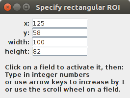
Create a UI: open a window to edit the position and dimensions of an ROI Here I illustrate how to create a user interface to accomplish a task that requires user input. Namely, how to edit the position (x, y) and dimensions (width, height) of an ImageJ rectangular ROI by typing in the precise integer values, or using arrows to increase/decrease the existing values, or using the scroll wheel to do the same. First, we define a RoiMaker class that extends KeyAdapter and implements the MouseWheelListener interface. The KeyAdapter class is a convenience class that implements all methods of the KeyListener interface, but where none of the methods do anything, sparing us from having to implement methods without a body. In RoiMaker, the constructor takes the list of all text fields to listen to (textfields: a total of four, for x, y, width, height of the ROI), and an index (ranging from 0 to 3) over that list, to determine which field to listen to. The parse method gets the text in the field and attempts to parse it as an integer. When it fails, the ROI is not updated, and the field is left painted with a red background. The Color returns back upon editing the value to a valid integer (actually, at every push of a key it will get set to white, and it is not set to red when parsing to an integer is successful). The update method attempts to parse the value in the text field, and can increment it (by 1 or -1, from the arrow keys), and if successful, updates the ROI on the active image. The keyReleased method overrides the homonimous method form the KeyAdapter, and implements the logic: if an arrow key is typed, increase or decrease by 1, accordingly; if any key is typed, just call update to parse the value and modify the ROI on the active image. Finally, the mouseWheelMoved method is from the MouseWheelListener interface, and is used to respond to events from the mouse wheel that happen over the text field. The wheel rotation is a positive or negative integer value, depending on the direction of rotation. Then we create the TextFieldUpdater class, which implements the RoiListener interface. Its only method roiModified provides an ImagePlus instance (imp) as argument, that we could use (but here we don't) to check whether a response is needed. Here, we ignore imp and respond no matter which value of imp is provided. We get the bounds from the ROI and update the content of the text fields. In this way, if the user manually drags the rectangular ROI around, or pulls its handles to change its dimensions or location, the textfields' values are updated. The CloseControl class extends WindowAdapter (similarly to how KeyAdapter implements empty methods for all methods of the KeyListener interface), and we implement only windowClosing: a method invoked when a window is closing, and which enables us to prevent its closing (by consuming the event), or to make it happen (by calling dispose() on the source of the event, which is the JFrame object (see below) that represents the whole window. Notice we ask the user, using a JOptionPane, to confirm whether the window should be closed--it is all too common to close a window by accidentally clicking the wrong button. With these classes in place, we declare the function specifyRoiUI which creates the window with text fields for manipulating the ROI position and dimensions, with all the event listeners that we declared above. The major abstraction here is that of a panel, with the class JPanel. A panel, like the panel in a figure of a scientific paper, is merely a bit of space: an area on the screen over which we define some behavior. How the content of the panel is laid out is managed here by a GridBagLayout: the most powerful--and to me, most intuitive and predictable--layout manager available in the java libraries. The GridBagLayout works as follows: for every UI element (a piece of text, a text field for entering text, a button, a panel (i.e. nested, a panel occupying a cell of another panel), etc.) to add to the panel, a set of constraints govern how the element is rendered (where, and in which dimensions). As its name indicates, the GridBagLayout is a grid, with each cell of the grid taking potentially different dimensions--but with all cells of the saw row having the same height, and all cells of the same column having the same width. The GridBagConstraints (here imported as GBC for brevity, with the variable gc pointing to an instance) contains a bunch of public, editable fields; when setting the constraints for an UI element, these are copied, so the gc object can continue to be edited, which facilitates e.g. sharing all constraints with the UI element next to the last added, except for e.g. its position in the X axis (i.e. by increasing the value of gc.gridx). In the for loop over the ["x", "y", "width", "height"] properties of a ROI's bounds, first a new JLabel is created, and then the value (read with the built-in function getattr to read an object's field by name) is used to create a new JTextField that will be used to edit it. Notice how the gc layout constraints are edited for each element (the label and the textfield) prior to adding them to the panel. The sequence is always the same: (1) create the UI element (e.g. a JTextField); (2) having adjusted the constraints (gc), call gb.setConstraints; and (3) add the UI element to the panel. Finally, a RoiMaker listener is created for each textfield, in order to respond to user input and update the ROI accordingly on the active image. Whenever a keyboard event or a mouse event occurs--actions initiated by the user--, the UI element will invoke the appropriate method of our listener, giving us the opportunity to react to the user's input. At the bottom, we add a doc to instruct the user on how to control the ROI position and dimensions using the keyboard and the mouse scroll wheel. Notice how we use gc.gridwidth = 2, to make the text span two horizontally adjacent cells instead of just one, and also we set gc.gridx = 0 to starting counting 2 cells from the first one, at index 0. Then, we instantiate a TextFieldUpdater (which implements RoiListener) and register it via Roi.addRoiListener, so that ImageJ will notify our class of any changes to an image's ROI, with our class then updating the text fields with the new values. E.g. if you were to drag the ROI, the first two fields, for the x, y position, would be updated. All that is left now is to define a JFrame that will contain our panel and offer buttons to e.g. close it or minimize it. The CloseControl class (see above) will manage whether the frame is closed (or not) upon clicking on its close button, and for that to work, we disable automatic closing first. Finally, we invoke the specifyRoiUI function to set it all up and show us our window. As final remarks, notice you could merely use Fiji's "Edit - Selection - Specify..." menu, which provides this functionality although not as interactive (it's a modal dialog, meaning, once open, no other window will respond to any input, and the dialog will remain on top always until closed). And notice as well that the ROI will be set on the active image: if the latter changes, the ROI--if any--of the active image will be replaced by the ROI specified by the position and dimension fields of this UI.
|
# Albert Cardona 2019-06-20
# Based on code written previously for lib/isoview_ui.py
from ij import IJ, ImagePlus, ImageListener
from ij.gui import RoiListener, Roi
from java.awt.event import KeyEvent, KeyAdapter, MouseWheelListener, WindowAdapter
from java.awt import Color, Rectangle, GridBagLayout, GridBagConstraints as GBC
from javax.swing import JFrame, JPanel, JLabel, JTextField, BorderFactory, JOptionPane
class RoiMaker(KeyAdapter, MouseWheelListener):
def __init__(self, textfields, index):
""" textfields: the list of 4 textfields for x,y,width and height.
index: of the textfields list, to chose the specific textfield to listen to. """
self.textfields = textfields
self.index = index
def parse(self):
""" Read the text in textfields[index] and parse it as a number.
When not a number, fail gracefully, print the error and paint the field red. """
try:
return int(self.textfields[self.index].getText())
except:
print "Can't parse integer from text: '%s'" % self.textfields[self.index].getText()
self.textfields[self.index].setBackground(Color.red)
def update(self, inc):
""" Set the rectangular ROI defined by the textfields values onto the active image. """
value = self.parse()
if value:
self.textfields[self.index].setText(str(value + inc))
imp = IJ.getImage()
if imp:
imp.setRoi(Roi(*[int(tf.getText()) for tf in self.textfields]))
def keyReleased(self, event):
""" If an arrow key is pressed, increase/decrese by 1.
If text is entered, parse it as a number or fail gracefully. """
self.textfields[self.index].setBackground(Color.white)
code = event.getKeyCode()
if KeyEvent.VK_UP == code or KeyEvent.VK_RIGHT == code:
self.update(1)
elif KeyEvent.VK_DOWN == code or KeyEvent.VK_LEFT == code:
self.update(-1)
else:
self.update(0)
def mouseWheelMoved(self, event):
""" Increase/decrese value by 1 according to the direction
of the mouse wheel rotation. """
self.update(- event.getWheelRotation())
class TextFieldUpdater(RoiListener):
def __init__(self, textfields):
self.textfields = textfields
def roiModified(self, imp, ID):
""" When the ROI of the active image changes, update the textfield values. """
if imp != IJ.getImage():
return # ignore if it's not the active image
roi = imp.getRoi()
if not roi or Roi.RECTANGLE != roi.getType():
return # none, or not a rectangle ROI
bounds = roi.getBounds()
if 0 == roi.getBounds().width + roi.getBounds().height:
bounds = Rectangle(0, 0, imp.getWidth(), imp.getHeight())
self.textfields[0].setText(str(bounds.x))
self.textfields[1].setText(str(bounds.y))
self.textfields[2].setText(str(bounds.width))
self.textfields[3].setText(str(bounds.height))
class CloseControl(WindowAdapter):
def __init__(self, roilistener):
self.roilistener = roilistener
def windowClosing(self, event):
answer = JOptionPane.showConfirmDialog(event.getSource(),
"Are you sure you want to close?",
"Confirm closing",
JOptionPane.YES_NO_OPTION)
if JOptionPane.NO_OPTION == answer:
event.consume() # Prevent closing
else:
Roi.removeRoiListener(self.roilistener)
event.getSource().dispose() # close the JFrame
def specifyRoiUI(roi=Roi(0, 0, 0, 0)):
# A panel in which to place UI elements
panel = JPanel()
panel.setBorder(BorderFactory.createEmptyBorder(10,10,10,10))
gb = GridBagLayout()
panel.setLayout(gb)
gc = GBC()
bounds = roi.getBounds() if roi else Rectangle()
textfields = []
roimakers = []
# Basic properties of most UI elements, will edit when needed
gc.gridx = 0 # can be any natural number
gc.gridy = 0 # idem.
gc.gridwidth = 1 # when e.g. 2, the UI element will occupy
# two horizontally adjacent grid cells
gc.gridheight = 1 # same but vertically
gc.fill = GBC.NONE # can also be BOTH, VERTICAL and HORIZONTAL
for title in ["x", "y", "width", "height"]:
# label
gc.gridx = 0
gc.anchor = GBC.EAST
label = JLabel(title + ": ")
gb.setConstraints(label, gc) # copies the given constraints 'gc',
# so we can modify and reuse gc later.
panel.add(label)
# text field, below the title
gc.gridx = 1
gc.anchor = GBC.WEST
text = str(getattr(bounds, title)) # same as e.g. bounds.x, bounds.width, ...
textfield = JTextField(text, 10) # 10 is the size of the field, in digits
gb.setConstraints(textfield, gc)
panel.add(textfield)
textfields.append(textfield) # collect all 4 created textfields for the listeners
# setup ROI and text field listeners
# (second argument is the index of textfield in the list of textfields)
listener = RoiMaker(textfields, len(textfields) -1)
roimakers.append(listener)
textfield.addKeyListener(listener)
textfield.addMouseWheelListener(listener)
# Position next ROI property in a new row
# by increasing the Y coordinate of the layout grid
gc.gridy += 1
# User documentation (uses HTML to define line breaks)
doc = JLabel("
|
||||||
|
Create a UI: searchable, tabulated view of file paths
In a research project running for some years the number of image files can grow to large numbers, often hundreds of thousands or milions. Because of the sheer number, these data sets are often stored in fileshares, mounted locally in your workstation via SMB or NFS. Often, searching for specific files in these data sets is slow, because the file system is slow or some other reason. To overcome this limitation, here we first run a shell one-liner script that writes all file paths into a text file, at one file path per line. Whenever the data set grows or changes, you'll have to re-run it:
$ find . -type f -printf "%p\n" > ~/Desktop/list.txt
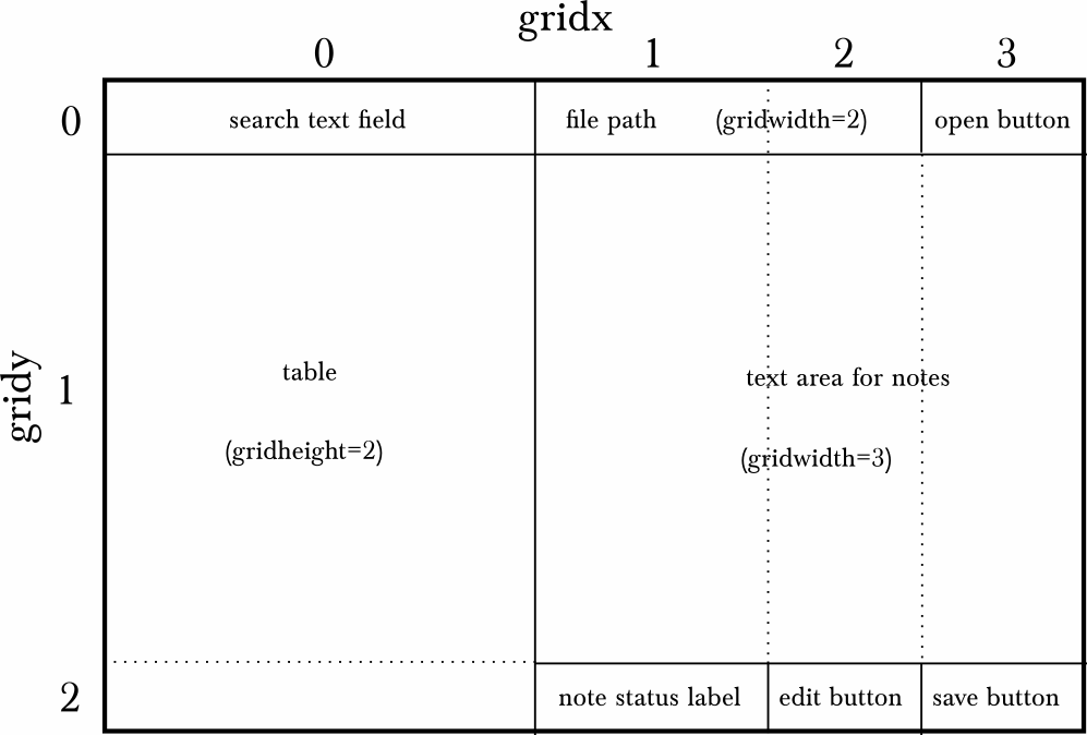
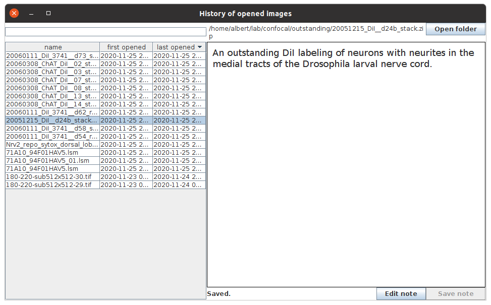
To run this python script, either just run it, and an OpenDialog will ask you for the text file with the file path list, or, update the txt_file variable to point to the file with the file paths. Once open, there's a search field at the top, and a table showing all file paths below. If the paths are relative (i.e. don't start with a '/' in *nix systems), fill in the text field at the bottom with the base path (the path to the directory that contains all the relative paths). Then, search: type in any text and push return. The listing of file paths will be reduced to those that contain the text. Alternatively, use a leading '/' in your text field to use regular expressions. Once the desired file is listed, double-click it: Fiji will open it, just as if you had drag and dropped it onto the Fiji/ImageJ toolbar, or had opened via "File - Open". The script first defines a TableModel, which is a class that extends AbstractTableModel. A model, in user interface parlance, is actually the data itself: a data structure that organizes the data in a predetermined way, following an interface contract (here, the homonymously named TableModel from the javax.swing package for building user interfaces). If you read the methods of class TableModel you'll notice methods for getting the number of columns and rows, and retrieving the data from a particular table cell, by index. All of these are methods required by the TableModel interface. I've added an additional method, filter, which, when invoked with a string as argument (named regex, but which can be plain text or, when starting with a '/', it's interpreted as a regular expression) will then shorten the list of stored file paths self.paths to merely those that match. The filtering is done in parallel using the Collections.parallelStream method that all java collections, including ArrayList (self.paths is an instance of ArrayList) implement. The class RowClickListener implements a listener for the mouse click on a row, obviously. This listener will later be added to the list of listeners of the table. The class EnterListener does just that for the search field. The class Closing is also a listener, but one that extends the WindowAdapter class to spare us from having to implement methods from the WindowListener interface that we won't use. This is a common pattern in java user interface libraries: a listener interface declares various methods, and then an adapter class that implements that interface exists, with empty implementations for all of the interface's methods, for convenience. The function makeUI binds it all together: creates the table, sets it up in a frame that also contains the regex_field where we'll type the search string, and the base_path_field for the base path string if needed. Then various JPanel organize these UI elements and a simple BoxLayout organizes where they render (see also another version of this script using GridBagLayout). Then instances of the various listeners are added to the table and fields. The launch function is a convenient wrapper for a run function that invokes makeUI with a given table model. Later, this isused to show the user interface from the event dispatch thread via SwingUtilities.invokeLater, as required for all UI-editing operations of the javax.swing library (see the "Swing's Threading Policy" at the bottom of this documentation). Turns out that all jython functions implement Runnable, the type expected by the sole argument of invokeLater, so instead of creating yet another class just to implement it, we use run instead. |
# A graphical user interface to keep track of files opened with Fiji
# and with the possibility of taking notes for each,
# which are persisted in a CSV file.
#
# Select a row to see its file path and note, if any.
# Double-click the file path to open the image corresponding to the selected table row.
# Click the "Open folder" to open the containing folder.
# Click the "Edit note" to start editing it, and "Save note" to sync to a CSV file.
#
# Albert Cardona 2020-11-22


from javax.swing import JPanel, JFrame, JTable, JScrollPane, JButton, JTextField, \
                        JTextArea, ListSelectionModel, SwingUtilities, JLabel, BorderFactory
from javax.swing.table import AbstractTableModel
from java.awt import GridBagLayout, GridBagConstraints, Dimension, Font, Insets, Color
from java.awt.event import KeyAdapter, MouseAdapter, KeyEvent, ActionListener, WindowAdapter
from javax.swing.event import ListSelectionListener
from java.lang import Thread, Integer, String, System
import os, csv, re
from datetime import datetime
from ij import ImageListener, ImagePlus, IJ, WindowManager
from ij.io import OpenDialog
from java.util.concurrent import Executors, TimeUnit
from java.util.concurrent.atomic import AtomicBoolean
from java.io import File


# EDIT here: where you want the CSV file to live.
# By default, lives in your user home directory as a hidden file.
csv_image_notes = os.path.join(System.getProperty("user.home"),
                               ".fiji-image-notes.csv")

# Generic read and write CSV functions
def openCSV(filepath, header_length=1):
  with open(filepath, 'r') as csvfile:
    reader = csv.reader(csvfile, delimiter=',', quotechar="\"")
    header_rows = [reader.next() for i in xrange(header_length)]
    rows = [columns for columns in reader]
    return header_rows, rows

def writeCSV(filepath, header, rows):
   """ filepath: where to write the CSV file
       header: list of header titles
       rows: list of lists of column values
       Writes first to a temporary file, and upon successfully writing it in full,
       then rename it to the target filepath, overwriting it.
   """
   with open(filepath + ".tmp", 'wb') as csvfile:
     w = csv.writer(csvfile, delimiter=',', quotechar="\"",
                    quoting=csv.QUOTE_NONNUMERIC)
     if header:
       w.writerow(header)
     for row in rows:
       w.writerow(row)
     # when written in full, replace the old one if any
     os.rename(filepath + ".tmp", filepath)

# Prepare main data structure: a list (rows) of lists (columns)
# Load the CSV file if it exists, otherwise use an empty data structure
if os.path.exists(csv_image_notes):
  header_rows, entries = openCSV(csv_image_notes, header_length=1)
  header = header_rows[0]
else:
  header = ["name", "first opened", "last opened", "filepath", "notes"]
  entries = []

# The subset of entries that are shown in the table (or all)
table_entries = entries

# Map of file paths vs. index of entries
image_paths = {row[3]: i for i, row in enumerate(entries)}

# A model (i.e. an interface to access the data) of the JTable listing all opened image files
class TableModel(AbstractTableModel):
  def getColumnName(self, col):
    return header[col]
  def getColumnClass(self, col): # for e.g. proper numerical sorting
    return String # all as strings
  def getRowCount(self):
    return len(table_entries)
  def getColumnCount(self):
    return len(header) -2 # don't show neither the full filepath nor the notes in the table
  def getValueAt(self, row, col):
    return table_entries[row][col]
  def isCellEditable(self, row, col):
    return False # none editable
  def setValueAt(self, value, row, col):
    pass # none editable


# Create the GUI: a 3-column table and a text area next to it
# to show and write notes for any selected row, plus some buttons and a search field
all = JPanel()
all.setBackground(Color.white)
gb = GridBagLayout()
all.setLayout(gb)
c = GridBagConstraints()

# Top-left element: a text field for filtering rows by regular expression match
c.gridx = 0
c.gridy = 0
c.anchor = GridBagConstraints.CENTER
c.fill = GridBagConstraints.HORIZONTAL
search_field = JTextField("")
gb.setConstraints(search_field, c)
all.add(search_field)

# Bottom left element: the table, wrapped in a scrollable component
table = JTable(TableModel())
table.setSelectionMode(ListSelectionModel.SINGLE_SELECTION)
#table.setCellSelectionEnabled(True)
table.setAutoCreateRowSorter(True) # to sort the view only, not the data in the underlying TableModel
c.gridx = 0
c.gridy = 1
c.anchor = GridBagConstraints.NORTHWEST
c.fill = GridBagConstraints.BOTH # resize with the frame
c.weightx = 1.0
c.gridheight = 2
jsp = JScrollPane(table)
jsp.setMinimumSize(Dimension(400, 500))
gb.setConstraints(jsp, c)
all.add(jsp)

# Top component: a text area showing the full file path to the image in the selected table row
c.gridx = 1
c.gridy = 0
c.gridheight = 1
c.gridwidth = 2
path = JTextArea("")
path.setEditable(False)
path.setMargin(Insets(4, 4, 4, 4))
path.setLineWrap(True)
path.setWrapStyleWord(True)
gb.setConstraints(path, c)
all.add(path)

# Top-right button to open the folder containing the image in the selected table row
c.gridx = 3
c.gridy = 0
c.gridwidth = 1
c.fill = GridBagConstraints.NONE
c.weightx = 0.0 # let the previous ('path') component stretch as much as possible
open_from_folder = JButton("Open folder")
gb.setConstraints(open_from_folder, c)
all.add(open_from_folder)

# Middle-right textarea showing the text of a note associated with the selected table row image
c.gridx = 1
c.gridy = 1
c.weighty = 1.0
c.gridwidth = 3
c.fill = GridBagConstraints.BOTH
textarea = JTextArea()
textarea.setBorder(BorderFactory.createCompoundBorder(
                    BorderFactory.createLineBorder(Color.BLACK),
                    BorderFactory.createEmptyBorder(10, 10, 10, 10)))
textarea.setLineWrap(True)
textarea.setWrapStyleWord(True) # wrap text by cutting lines at whitespace
textarea.setEditable(False)
font = textarea.getFont().deriveFont(18.0)
textarea.setFont(font)
textarea.setPreferredSize(Dimension(500, 500))
gb.setConstraints(textarea, c)
all.add(textarea)

# Bottom text label showing the status of the note: whether it's being edited, or saved.
c.gridx = 1
c.gridy = 2
c.gridwidth = 1
c.weightx = 0.5
c.weighty = 0.0
note_status = JLabel("")
gb.setConstraints(note_status, c)
all.add(note_status)

# 2nd-to-last Bottom right button for editing the note text in the middle-right text area
c.gridx = 2
c.gridy = 2
c.weightx = 0.0
c.anchor = GridBagConstraints.NORTHEAST
edit_note = JButton("Edit note")
edit_note.setEnabled(False)
gb.setConstraints(edit_note, c)
all.add(edit_note)

# Bottom right button for requesting that the text note in the text area be saved to the CSV file
c.gridx = 3
c.gridy = 2
save_note = JButton("Save note")
save_note.setEnabled(False)
gb.setConstraints(save_note, c)
all.add(save_note)

frame = JFrame("History of opened images")
frame.getContentPane().add(all)
frame.pack()
frame.setVisible(True)


# Wire up the buttons and fields with functions

# Convert from row index in the view (could e.g. be sorted)
# to the index in the underlying table model
def getSelectedRowIndex():
  viewIndex = table.getSelectionModel().getLeadSelectionIndex()
  modelIndex = table.convertRowIndexToModel(viewIndex)
  return modelIndex

# For regular expression-based filtering of the table rows
def filterTable():
  global table_entries # flag global variable as one to modify here
  try:
    text = search_field.getText()
    if 0 == len(text):
      table_entries = entries # reset: show all rows
    else:
      pattern = re.compile(text)
      # Search in filepath and notes
      table_entries = [row for row in entries if pattern.search(row[-2]) or pattern.search(row[-1])]
    SwingUtilities.invokeLater(lambda: table.updateUI()) # executed by the event dispatch thread
  except:
    print "Malformed regex pattern"

class TypingInSearchField(KeyAdapter):
  def keyPressed(self, event):
    if KeyEvent.VK_ENTER == event.getKeyCode():
      filterTable()
    elif KeyEvent.VK_ESCAPE == event.getKeyCode():
      search_field.setText("")
      filterTable() # to restore the full list of rows

search_field.addKeyListener(TypingInSearchField())


# Function for the button to open the folder containing the image file path in the selected table row
class OpenAtFolder(ActionListener):
  def actionPerformed(self, event):
    if 0 == path.getText().find("http"):
      IJ.showMessage("Can't open folder: it's an URL")
      return
    directory = os.path.dirname(path.getText())
    od = OpenDialog("Open", directory, None)
    filepath = od.getPath()
    if filepath:
      IJ.open(filepath)

open_from_folder.addActionListener(OpenAtFolder())


# Function for the button to enable editing the note for the selected table row
class ClickEditButton(ActionListener):
  def actionPerformed(self, event):
    edit_note.setEnabled(False)
    save_note.setEnabled(True)
    note_status.setText("Editing...")
    textarea.setEditable(True)
    textarea.requestFocus()

edit_note.addActionListener(ClickEditButton())

# Function for the bottom right button to request saving the text note to the CSV file
def requestSave(rowIndex=None):
  # Update table model data
  rowIndex = getSelectedRowIndex() if rowIndex is None else rowIndex
  table_entries[rowIndex][-1] = textarea.getText()
  # Signal synchronize to disk next time the scheduled thread wakes up
  requested_save_csv.set(True)

class RequestSave(ActionListener):
  def actionPerformed(self, event):
    requestSave()

save_note.addActionListener(RequestSave())


# Flag to set to True to request the table model data be saved to the CSV file
requested_save_csv = AtomicBoolean(False)

# A function to save the table to disk in CSV format.
# Checks if the requested_save_csv flag was set, and if so, writes the CSV file.
def saveTable():
  def after():
    # UI elements to alter under the event dispatch thread
    note_status.setText("Saved.")
    edit_note.setEnabled(True)
    save_note.setEnabled(False)
  # Repeatedly attempt to write the CSV until there are no more updates,
  # in which case the scheduled thread (see below) will pause for a bit before retrying.
  while requested_save_csv.getAndSet(False):
    writeCSV(csv_image_notes, header, entries)
    SwingUtilities.invokeLater(after)

# Every 500 milliseconds, save to CSV only if it has been requested
# This background thread is shutdown when the JFrame window is closed
exe = Executors.newSingleThreadScheduledExecutor()
exe.scheduleAtFixedRate(saveTable, 0, 500, TimeUnit.MILLISECONDS)

# When selecting a different table row or closing the window
# and changes weren't saved, ask whether to save them,
# and in any case print them to the ImageJ log window to make them recoverable.
def askToSaveUnsavedChanges(rowIndex):
  if note_status.getText() == "Unsaved changes.":
    if IJ.showMessageWithCancel("Alert", "Save current note?"):
      requestSave(rowIndex=rowIndex)
    else:
      # Stash current note in the log window
      IJ.log("Discarded note for image at:")
      IJ.log(path.getText())
      IJ.log(textarea.getText())
      IJ.log("===")

# Function to run upon closing the window
class Cleanup(WindowAdapter):
  def windowClosing(self, event):
    askToSaveUnsavedChanges(getSelectedRowIndex())
    exe.shutdown()
    ImagePlus.removeImageListener(open_imp_listener)
    event.getSource().dispose() # same as frame.dispose()

frame.addWindowListener(Cleanup())


def addOrUpdateEntry(imp):
  """
  This function runs in response to an image being opened,
  and finds out whether a new entry should be added to the table (and CSV file)
  or whether an existing entry ought to be added,
  or whether there's nothing to do because it's a new image not opened from a file.

  imp: an ImagePlus
  """
  # Was the image opened from a file?
  fi = imp.getOriginalFileInfo()
  if not fi:
    # Image was created new, not from a file: ignore
    return
  filepath =  os.path.join(fi.directory, fi.fileName) if not fi.url else fi.url
  # Had we opened this file before?
  index = image_paths.get(filepath, None)
  now = datetime.now().strftime("%Y-%m-%d %H:%M")
  if index is None:
    # File isn't yet in the table: add it
    entries.append([fi.fileName, now, now, filepath, ""])
    image_paths[filepath] = len(entries) -1
  else:
    # File exists: edit its last seen date
    entries[index][2] = now
  # Rerun filtering if needed
  filterTable()
  # Update table to reflect changes to the underlying data model
  def repaint():
    table.updateUI()
    table.repaint()
  SwingUtilities.invokeLater(repaint) # must run in the event dispatch thread
  # Request writing changes to the CSV file
  requested_save_csv.set(True)

# A listener to react to images being opened via an ij.io.Opener from e.g. "File - Open"
class OpenImageListener(ImageListener):
  def imageClosed(self, imp):
    pass
  def imageUpdated(self, imp):
    pass
  def imageOpened(self, imp):
    addOrUpdateEntry(imp)

open_imp_listener = OpenImageListener() # keep a reference for unregistering on window closing
ImagePlus.addImageListener(open_imp_listener)

# A listener to detect whether there have been any edits to the text note
class TypingListener(KeyAdapter):
  def keyPressed(self, event):
    rowIndex = getSelectedRowIndex()
    if event.getSource().getText() != table_entries[rowIndex][-1]:
      note_status.setText("Unsaved changes.")

textarea.addKeyListener(TypingListener())


# React to a row being selected by showing the corresponding note
# in the textarea to the right
class TableSelectionListener(ListSelectionListener):
  def __init__(self):
    self.lastRowIndex = -1
  def valueChanged(self, event):
    if event.getValueIsAdjusting():
      return
    rowIndex = getSelectedRowIndex()
    print "rowIndex:", rowIndex, "last:", self.lastRowIndex
    if -1 != self.lastRowIndex and rowIndex != self.lastRowIndex:
      askToSaveUnsavedChanges(self.lastRowIndex)
    self.lastRowIndex = rowIndex
    # Must run later in the context of the event dispatch thread
    # when the latter has updated the table selection
    def after():
      path.setText(table_entries[rowIndex][-2])
      path.setToolTipText(path.getText()) # for mouse over to show full path
      textarea.setText(table_entries[rowIndex][-1])
      textarea.setEditable(False)
      edit_note.setEnabled(True)
      save_note.setEnabled(False)
      note_status.setText("Saved.") # as in entries and the CSV file
    SwingUtilities.invokeLater(after)

table.getSelectionModel().addListSelectionListener(TableSelectionListener())

# Open an image on double-clicking the filepath label
# but merely bring its window to the front if it's already open:
class PathOpener(MouseAdapter):
  def mousePressed(self, event):
    if 2 == event.getClickCount():
      # If the file is open, bring it to the front
      ids = WindowManager.getIDList()
      if ids: # can be null
        is_open = False # to allow bringing to front more than one window
                        # in cases where it has been opened more than once
        for ID in ids:
          imp = WindowManager.getImage(ID)
          fi = imp.getOriginalFileInfo()
          filepath = os.path.join(fi.directory, fi.fileName)
          if File(filepath).equals(File(event.getSource().getText())):
            imp.getWindow().toFront()
            is_open = True
        if is_open:
          return
      # otherwise open it
      IJ.open(table_entries[getSelectedRowIndex()][-2])

path.addMouseListener(PathOpener())

# Enable changing text font size in all components by control+shift+(plus|equals)/minus
components = list(all.getComponents()) + [table, table.getTableHeader()]
class FontSizeAdjuster(KeyAdapter):
  def keyPressed(self, event):
    if event.isControlDown() and event.isShiftDown(): # like in e.g. a web browser
      sign = {KeyEvent.VK_MINUS: -1,
              KeyEvent.VK_PLUS: 1,
              KeyEvent.VK_EQUALS: 1}.get(event.getKeyCode(), 0)
      if 0 == sign: return
      # Adjust font size of all UI components
      for component in components:
        font = component.getFont()
        if not font: continue
        size = max(8.0, font.getSize2D() + sign * 0.5)
        if size != font.getSize2D():
          component.setFont(font.deriveFont(size))
      def repaint():
        # Adjust the height of a JTable's rows (why it doesn't do so automatically is absurd)
        if table.getRowCount() > 0:
          r = table.prepareRenderer(table.getCellRenderer(0, 1), 0, 1)
          table.setRowHeight(max(table.getRowHeight(), r.getPreferredSize().height))
      SwingUtilities.invokeLater(repaint)

for component in components:
  component.addKeyListener(FontSizeAdjuster())
|
||||||
|
Table with annotated history of opened image files
When browsing through a large collection of e.g. confocal stacks, we do so purposefully: to find a particular feature in the imaged volume, or to classify stacks as having certain conditions. While we can, and often do, keep such notes elsewhere in a spreadsheet or a text document, by doing so our notes are disconnected from the image data. Coping mechanisms include copy-pasting file paths, but that becomes cumbersome. For extremely large collections with multiple users annotating simultaneously, there exist specialized applications (e.g. CATMAID for annotating, grouping and classifying confocal stacks; Dunst et al. 2015.). But for intermediate collections of hundreds or thousands of stacks that a single researcher generates or analyzes, we can come up with a solution with a minimal learning curve and requiring no installation or maintenance effort, that is also trivial to backup or share with others. Here, I show how to keep track of opened image files and to store our notes on each opened image, while also recording when the image was first and last opened. With this approach, multi-day image browsing and analysis sessions are possible, picking up from where we last left it at. The list of opened images is shown in a table (an all-powerful JTable), at one image per row along with the first opened and last opened date, with all three columns being sortable (click the header of each column and a black arrow will appear pointing up or down if you click a second time). Note that the columns are resizable by click and drag on the vertical line between the column headers. Upon selecting a row, the file path for that image is shown in the upper right text area, and our notes on the file, if any, are shown in a large text area to the right. To reopen a previously seen image, double-click on its file path. If the image is already open but it's minimized or hidden behind other images, its image window will be brought to the front. To open more images from the same folder, push the "Open folder" button. To start editing the note, push the "Edit note" button; to save the note, push "Save note". The status text label under the note text area will show us whether the note is already saved or is being edited. If we were to close the window, or select a different table row (which would replace the note with the corresponding note), it will ask us whether we want to save any unsaved changes to that note. The entire table, file paths and corresponding notes are saved in a CSV file. In practice, you'd create a different CSV file (by editing the csv_image_notes variable, or replacing it with an OpenDialog to request a new file from the user every time the script is run. But in any case, for large collections you may end up with thousands of entries. To find specific images that you annotated, the text field at the top of the table lets you search, with regular expressions, into both the file paths and the notes, limiting the rows shown in the table to those that match the search pattern. To clear the search, push the ESC key, or delete any text in the search field and push enter, both approaches restoring the view to the whole content of the table. For the layout of all graphical user interface components we use a GridBagLayout, in this configuration:
The key to understanding the layout is to realize that it defines a grid (hence the name), whose cells are zero-indexed by the gridx and gridy variables of the GridBagConstraints instance (named c) used for gb.setConstraints to specify, for each component, where it is to be placed in the all JPanel, and importantly, how each component is to behave: some take three columns (i.e. c.gridwidth = 3), some take two rows (i.e. c.gridheight = 2). And some are not to be resized (i.e. c.fill = GridBagConstraints.NONE), and some should fill up as much space as is available (i.e. c.fill = GridBagConstraints.BOTH, with other options being HORIZONTAL or VERTICAL). To make some components take up as much space as possible, we give them a c.weightx = 1.0 or c.weighty = 1.0. The c.anchor is used to specify where, within the available cell space, should the component be rendered if it is not to fill the whole space, with e.g. top-left being GridBagConstraints.NORTHWEST. A critical feature to undertand the code for setting the constraints to each UI component is that the gb.setConstraints method call uses the GridBagConstraints c instance as provided at that moment, copying its contents and storing it for that specific component. Further modifications to the fields of c won't have any effect on previously constrained components. This allows a style of coding in which we only adjust, from c, the fields that change (e.g. increasing gridx). In this example, for clarity, I specified for each component the gridx and gridy, but not all the others which tend to change a lot less (c.anchor, c.fill, c.weightx etc.), changing only those that are different from the previously added cell. Also, while I added UI components from left to right and top to bottom, the order in which they are added doesn't matter.
After defining the whole GUI, which is complete by adding the all panel to the JFrame, then we define a number of listener classes to wiring up the search_field, the table selection and the buttons with functions. Note that we could have defined most of these listeners as keyword arguments in the UI component constructor invocations, e.g. something like actionPerformed=saveTable, but I chose not to follow this approach, as it would have required defining functions prior to defining UI elements (the functions that act as targets of the various listeners have to exist at that point). Given that each of these listeners invokes methods on other UI components, the code would have been spaghetti (in other words a confusing mess, with functions using global variables defined later in the script; see the spaghetti version of this example script). Also, notice the use of the static method SwingUtilities.invokeLater whenever there is to be an update to the graphical user interface. We first define a small function (often I've named it after) that does all the updating (enabling buttons, changing text, etc., all of which will result in redrawing the GUI in the screen) and, taking advantage of the fact that all jython functions implement the Runnable interface, request via SwingUtilities.invokeLater that the function be invoked at a later time by the event dispatch thread. "Swing" being merely the name of the graphical user interface library that we are using here. Updating GUI components in a thread other than the event dispatch thread (such as the thread that Fiji uses to open images, or the script editor's execution thread) can result in an incorrectly or incompletely rendered window. If that was to happen, almost always all you'd need is to resize the window with the mouse to force a redraw, which would correct any rendering issues. When using a JTable, be mindful of the difference between how the table looks (e.g. are the rows sorted, or filtered) and the underlying data structure (table_entries). In this script there are:
Another feature to notice is the use of the global built-in keyword in the function filterTable, to indicate that the global variable table_entries will be modified in this function. Without the global keyword, a variable named table_entries defined within the function would be a different, local variable. While all global variables can be read from a function, to modify them they must be tagged with global right at the beginning of the function declaration. For saving the CSV file, notice it is done indirectly to avoid blocking the event dispatch thread that updates and operates the graphical user interface while a potentially time-consuming operation such as writing a file to disk is ongoing. The function requestSave edits the table_entries at the appropriate row and column to update the note associated with that image, but then, instead of writing the changes to the CSV file, instead sets the requested_save_csv to true. This is an AtomicBoolean: an object that wraps a boolean value (true or false) which synchronizes access to the value, so that only one thread at a time can do so. Then, in the background, there is an ScheduledExecutorService (the exe) that invokes the saveTable function periodically every 500 milliseconds. While the requested_save_csv flag is set (could be set again to true upon finishing writing the CSV file, so we do continue checking in a loop until it is false and the loop ends), the entries are written to the CSV file via writeCSV, which overwrites any existing CSV file at the file path denoted by csv_image_notes. After another 500 milliseconds, the scheduled task wakes up again and checks again whether the flag is set to true. In the event of success in writing the CSV file, the note_status and associated buttons are updated. The function addOrUpdateEntry takes an ImagePlus as argument and checks if its associated file path (as specified in its FileInfo). If the file had been seen before, merely update the last seen timestamp, otherwise append it to the tbable. And in any case request that the CSV file is saved. This function is then called from an ImageListener named OpenImageListener, where its imageOpened method does the work. This listener is hooked in via the static method ImagePlus.addImageListener, so that Fiji will invoke our code whenever a new image is opened via its Opener system (which underlies the IJ.open and IJ.openImage static methods frequently used in scripts and plugins, and also the menu "File - Open"). Finally, I've added here the class FontSizeAdjuster which is a listener for keyboard events that is added to all GUI components. Whenever control+shift+<plus|equals|minus> key combination are pressed, the font size of all components will be adjusted accordingly. This helps for e.g. high DPI screens where the default font may be too small. |
# A graphical user interface to keep track of files opened with Fiji
# and with the possibility of taking notes for each,
# which are persisted in a CSV file.
#
# Select a row to see its file path and note, if any.
# Double-click the file path to open the image corresponding to the selected table row.
# Click the "Open folder" to open the containing folder.
# Click the "Edit note" to start editing it, and "Save note" to sync to a CSV file.
#
# Albert Cardona 2020-11-22


from javax.swing import JPanel, JFrame, JTable, JScrollPane, JButton, JTextField, \
                        JTextArea, ListSelectionModel, SwingUtilities, JLabel, BorderFactory
from javax.swing.table import AbstractTableModel
from java.awt import GridBagLayout, GridBagConstraints, Dimension, Font, Insets, Color
from java.awt.event import KeyAdapter, MouseAdapter, KeyEvent, ActionListener, WindowAdapter
from javax.swing.event import ListSelectionListener
from java.lang import Thread, Integer, String, System
import os, csv, re
from datetime import datetime
from ij import ImageListener, ImagePlus, IJ, WindowManager
from ij.io import OpenDialog
from java.util.concurrent import Executors, TimeUnit
from java.util.concurrent.atomic import AtomicBoolean
from java.io import File


# EDIT here: where you want the CSV file to live.
# By default, lives in your user home directory as a hidden file.
csv_image_notes = os.path.join(System.getProperty("user.home"),
                               ".fiji-image-notes.csv")

# Generic read and write CSV functions
def openCSV(filepath, header_length=1):
  with open(filepath, 'r') as csvfile:
    reader = csv.reader(csvfile, delimiter=',', quotechar="\"")
    header_rows = [reader.next() for i in xrange(header_length)]
    rows = [columns for columns in reader]
    return header_rows, rows

def writeCSV(filepath, header, rows):
   """ filepath: where to write the CSV file
       header: list of header titles
       rows: list of lists of column values
       Writes first to a temporary file, and upon successfully writing it in full,
       then rename it to the target filepath, overwriting it.
   """
   with open(filepath + ".tmp", 'wb') as csvfile:
     w = csv.writer(csvfile, delimiter=',', quotechar="\"",
                    quoting=csv.QUOTE_NONNUMERIC)
     if header:
       w.writerow(header)
     for row in rows:
       w.writerow(row)
     # when written in full, replace the old one if any
     os.rename(filepath + ".tmp", filepath)

# Prepare main data structure: a list (rows) of lists (columns)
# Load the CSV file if it exists, otherwise use an empty data structure
if os.path.exists(csv_image_notes):
  header_rows, entries = openCSV(csv_image_notes, header_length=1)
  header = header_rows[0]
else:
  header = ["name", "first opened", "last opened", "filepath", "notes"]
  entries = []

# The subset of entries that are shown in the table (or all)
table_entries = entries

# Map of file paths vs. index of entries
image_paths = {row[3]: i for i, row in enumerate(entries)}

# A model (i.e. an interface to access the data) of the JTable listing all opened image files
class TableModel(AbstractTableModel):
  def getColumnName(self, col):
    return header[col]
  def getColumnClass(self, col): # for e.g. proper numerical sorting
    return String # all as strings
  def getRowCount(self):
    return len(table_entries)
  def getColumnCount(self):
    return len(header) -2 # don't show neither the full filepath nor the notes in the table
  def getValueAt(self, row, col):
    return table_entries[row][col]
  def isCellEditable(self, row, col):
    return False # none editable
  def setValueAt(self, value, row, col):
    pass # none editable


# Create the GUI: a 3-column table and a text area next to it
# to show and write notes for any selected row, plus some buttons and a search field
all = JPanel()
all.setBackground(Color.white)
gb = GridBagLayout()
all.setLayout(gb)
c = GridBagConstraints()

# Top-left element: a text field for filtering rows by regular expression match
c.gridx = 0
c.gridy = 0
c.anchor = GridBagConstraints.CENTER
c.fill = GridBagConstraints.HORIZONTAL
search_field = JTextField("")
gb.setConstraints(search_field, c)
all.add(search_field)

# Bottom left element: the table, wrapped in a scrollable component
table = JTable(TableModel())
table.setSelectionMode(ListSelectionModel.SINGLE_SELECTION)
#table.setCellSelectionEnabled(True)
table.setAutoCreateRowSorter(True) # to sort the view only, not the data in the underlying TableModel
c.gridx = 0
c.gridy = 1
c.anchor = GridBagConstraints.NORTHWEST
c.fill = GridBagConstraints.BOTH # resize with the frame
c.weightx = 1.0
c.gridheight = 2
jsp = JScrollPane(table)
jsp.setMinimumSize(Dimension(400, 500))
gb.setConstraints(jsp, c)
all.add(jsp)

# Top component: a text area showing the full file path to the image in the selected table row
c.gridx = 1
c.gridy = 0
c.gridheight = 1
c.gridwidth = 2
path = JTextArea("")
path.setEditable(False)
path.setMargin(Insets(4, 4, 4, 4))
path.setLineWrap(True)
path.setWrapStyleWord(True)
gb.setConstraints(path, c)
all.add(path)

# Top-right button to open the folder containing the image in the selected table row
c.gridx = 3
c.gridy = 0
c.gridwidth = 1
c.fill = GridBagConstraints.NONE
c.weightx = 0.0 # let the previous ('path') component stretch as much as possible
open_from_folder = JButton("Open folder")
gb.setConstraints(open_from_folder, c)
all.add(open_from_folder)

# Middle-right textarea showing the text of a note associated with the selected table row image
c.gridx = 1
c.gridy = 1
c.weighty = 1.0
c.gridwidth = 3
c.fill = GridBagConstraints.BOTH
textarea = JTextArea()
textarea.setBorder(BorderFactory.createCompoundBorder(
                    BorderFactory.createLineBorder(Color.BLACK),
                    BorderFactory.createEmptyBorder(10, 10, 10, 10)))
textarea.setLineWrap(True)
textarea.setWrapStyleWord(True) # wrap text by cutting lines at whitespace
textarea.setEditable(False)
font = textarea.getFont().deriveFont(18.0)
textarea.setFont(font)
textarea.setPreferredSize(Dimension(500, 500))
gb.setConstraints(textarea, c)
all.add(textarea)

# Bottom text label showing the status of the note: whether it's being edited, or saved.
c.gridx = 1
c.gridy = 2
c.gridwidth = 1
c.weightx = 0.5
c.weighty = 0.0
note_status = JLabel("")
gb.setConstraints(note_status, c)
all.add(note_status)

# 2nd-to-last Bottom right button for editing the note text in the middle-right text area
c.gridx = 2
c.gridy = 2
c.weightx = 0.0
c.anchor = GridBagConstraints.NORTHEAST
edit_note = JButton("Edit note")
edit_note.setEnabled(False)
gb.setConstraints(edit_note, c)
all.add(edit_note)

# Bottom right button for requesting that the text note in the text area be saved to the CSV file
c.gridx = 3
c.gridy = 2
save_note = JButton("Save note")
save_note.setEnabled(False)
gb.setConstraints(save_note, c)
all.add(save_note)

frame = JFrame("History of opened images")
frame.getContentPane().add(all)
frame.pack()
frame.setVisible(True)


# Wire up the buttons and fields with functions

# Convert from row index in the view (could e.g. be sorted)
# to the index in the underlying table model
def getSelectedRowIndex():
  viewIndex = table.getSelectionModel().getLeadSelectionIndex()
  modelIndex = table.convertRowIndexToModel(viewIndex)
  return modelIndex

# For regular expression-based filtering of the table rows
def filterTable():
  global table_entries # flag global variable as one to modify here
  try:
    text = search_field.getText()
    if 0 == len(text):
      table_entries = entries # reset: show all rows
    else:
      pattern = re.compile(text)
      # Search in filepath and notes
      table_entries = [row for row in entries if pattern.search(row[-2]) or pattern.search(row[-1])]
    SwingUtilities.invokeLater(lambda: table.updateUI()) # executed by the event dispatch thread
  except:
    print "Malformed regex pattern"

class TypingInSearchField(KeyAdapter):
  def keyPressed(self, event):
    if KeyEvent.VK_ENTER == event.getKeyCode():
      filterTable()
    elif KeyEvent.VK_ESCAPE == event.getKeyCode():
      search_field.setText("")
      filterTable() # to restore the full list of rows

search_field.addKeyListener(TypingInSearchField())


# Function for the button to open the folder containing the image file path in the selected table row
class OpenAtFolder(ActionListener):
  def actionPerformed(self, event):
    if 0 == path.getText().find("http"):
      IJ.showMessage("Can't open folder: it's an URL")
      return
    directory = os.path.dirname(path.getText())
    od = OpenDialog("Open", directory, None)
    filepath = od.getPath()
    if filepath:
      IJ.open(filepath)

open_from_folder.addActionListener(OpenAtFolder())


# Function for the button to enable editing the note for the selected table row
class ClickEditButton(ActionListener):
  def actionPerformed(self, event):
    edit_note.setEnabled(False)
    save_note.setEnabled(True)
    note_status.setText("Editing...")
    textarea.setEditable(True)
    textarea.requestFocus()

edit_note.addActionListener(ClickEditButton())

# Function for the bottom right button to request saving the text note to the CSV file
def requestSave():
  # Update table model data
  rowIndex = getSelectedRowIndex()
  table_entries[rowIndex][-1] = textarea.getText()
  # Signal synchronize to disk next time the scheduled thread wakes up
  requested_save_csv.set(True)

class RequestSave(ActionListener):
  def actionPerformed(self, event):
    requestSave()

save_note.addActionListener(RequestSave())


# Flag to set to True to request the table model data be saved to the CSV file
requested_save_csv = AtomicBoolean(False)

# A function to save the table to disk in CSV format.
# Checks if the requested_save_csv flag was set, and if so, writes the CSV file.
def saveTable():
  def after():
    # UI elements to alter under the event dispatch thread
    note_status.setText("Saved.")
    edit_note.setEnabled(True)
    save_note.setEnabled(False)
  # Repeatedly attempt to write the CSV until there are no more updates,
  # in which case the scheduled thread (see below) will pause for a bit before retrying.
  while requested_save_csv.getAndSet(False):
    writeCSV(csv_image_notes, header, entries)
    SwingUtilities.invokeLater(after)

# Every 500 milliseconds, save to CSV only if it has been requested
# This background thread is shutdown when the JFrame window is closed
exe = Executors.newSingleThreadScheduledExecutor()
exe.scheduleAtFixedRate(saveTable, 0, 500, TimeUnit.MILLISECONDS)

# When selecting a different table row or closing the window
# and changes weren't saved, ask whether to save them,
# and in any case print them to the ImageJ log window to make them recoverable.
def askToSaveUnsavedChanges():
  if note_status.getText() == "Unsaved changes.":
    if IJ.showMessageWithCancel("Alert", "Save current note?"):
      requestSave()
    else:
      # Stash current note in the log window
      IJ.log("Discarded note for image at:")
      IJ.log(path.getText())
      IJ.log(textarea.getText())
      IJ.log("===")

# Function to run upon closing the window
class Cleanup(WindowAdapter):
  def windowClosing(self, event):
    askToSaveUnsavedChanges()
    exe.shutdown()
    ImagePlus.removeImageListener(open_imp_listener)
    event.getSource().dispose() # same as frame.dispose()

frame.addWindowListener(Cleanup())


def addOrUpdateEntry(imp):
  """
  This function runs in response to an image being opened,
  and finds out whether a new entry should be added to the table (and CSV file)
  or whether an existing entry ought to be added,
  or whether there's nothing to do because it's a new image not opened from a file.

  imp: an ImagePlus
  """
  # Was the image opened from a file?
  fi = imp.getOriginalFileInfo()
  if not fi:
    # Image was created new, not from a file: ignore
    return
  filepath =  os.path.join(fi.directory, fi.fileName) if not fi.url else fi.url
  # Had we opened this file before?
  index = image_paths.get(filepath, None)
  now = datetime.now().strftime("%Y-%m-%d %H:%M")
  if index is None:
    # File isn't yet in the table: add it
    entries.append([fi.fileName, now, now, filepath, ""])
    image_paths[filepath] = len(entries) -1
  else:
    # File exists: edit its last seen date
    entries[index][2] = now
  # Rerun filtering if needed
  filterTable()
  # Update table to reflect changes to the underlying data model
  def repaint():
    table.updateUI()
    table.repaint()
  SwingUtilities.invokeLater(repaint) # must run in the event dispatch thread
  # Request writing changes to the CSV file
  requested_save_csv.set(True)

# A listener to react to images being opened via an ij.io.Opener from e.g. "File - Open"
class OpenImageListener(ImageListener):
  def imageClosed(self, imp):
    pass
  def imageUpdated(self, imp):
    pass
  def imageOpened(self, imp):
    addOrUpdateEntry(imp)

open_imp_listener = OpenImageListener() # keep a reference for unregistering on window closing
ImagePlus.addImageListener(open_imp_listener)

# A listener to detect whether there have been any edits to the text note
class TypingListener(KeyAdapter):
  def keyPressed(self, event):
    rowIndex = getSelectedRowIndex()
    if event.getSource().getText() != table_entries[rowIndex][-1]:
      note_status.setText("Unsaved changes.")

textarea.addKeyListener(TypingListener())


# React to a row being selected by showing the corresponding note
# in the textarea to the right
class TableSelectionListener(ListSelectionListener):
  def valueChanged(self, event):
    if event.getValueIsAdjusting():
      return
    askToSaveUnsavedChanges()
    # Must run later in the context of the event dispatch thread
    # when the latter has updated the table selection
    def after():
      rowIndex = getSelectedRowIndex()
      print "rowIndex:", rowIndex
      path.setText(table_entries[rowIndex][-2])
      path.setToolTipText(path.getText()) # for mouse over to show full path
      textarea.setText(table_entries[rowIndex][-1])
      textarea.setEditable(False)
      edit_note.setEnabled(True)
      save_note.setEnabled(False)
      note_status.setText("Saved.") # as in entries and the CSV file
    SwingUtilities.invokeLater(after)

table.getSelectionModel().addListSelectionListener(TableSelectionListener())

# Open an image on double-clicking the filepath label
# but merely bring its window to the front if it's already open:
class PathOpener(MouseAdapter):
  def mousePressed(self, event):
    if 2 == event.getClickCount():
      # If the file is open, bring it to the front
      ids = WindowManager.getIDList()
      if ids: # can be null
        is_open = False # to allow bringing to front more than one window
                        # in cases where it has been opened more than once
        for ID in ids:
          imp = WindowManager.getImage(ID)
          fi = imp.getOriginalFileInfo()
          filepath = os.path.join(fi.directory, fi.fileName)
          if File(filepath).equals(File(event.getSource().getText())):
            imp.getWindow().toFront()
            is_open = True
        if is_open:
          return
      # otherwise open it
      IJ.open(table_entries[getSelectedRowIndex()][-2])

path.addMouseListener(PathOpener())

# Enable changing text font size in all components by control+shift+(plus|equals)/minus
components = list(all.getComponents()) + [table, table.getTableHeader()]
class FontSizeAdjuster(KeyAdapter):
  def keyPressed(self, event):
    if event.isControlDown() and event.isShiftDown(): # like in e.g. a web browser
      sign = {KeyEvent.VK_MINUS: -1,
              KeyEvent.VK_PLUS: 1,
              KeyEvent.VK_EQUALS: 1}.get(event.getKeyCode(), 0)
      if 0 == sign: return
      # Adjust font size of all UI components
      for component in components:
        font = component.getFont()
        if not font: continue
        size = max(8.0, font.getSize2D() + sign * 0.5)
        if size != font.getSize2D():
          component.setFont(font.deriveFont(size))
      def repaint():
        # Adjust the height of a JTable's rows (why it doesn't do so automatically is absurd)
        if table.getRowCount() > 0:
          r = table.prepareRenderer(table.getCellRenderer(0, 1), 0, 1)
          table.setRowHeight(max(table.getRowHeight(), r.getPreferredSize().height))
      SwingUtilities.invokeLater(repaint)

for component in components:
  component.addKeyListener(FontSizeAdjuster())
|
||||||
|
Hot corners: run ImageJ commands when the mouse visits a screen corner
In this example, I illustrate how to react to mouse movement by keeping track of where the mouse is, and querying whether the mouse position falls within a predetermined area, such as a corner, that has been associated with an action. First we get the screen dimensions by asking the Toolkit, which is a class with methods for finding out system properties that relate to the graphical interface (as opposed to System, whose methods provide access to system services and capabilities). The corners is a dictionary whose keys are the name of the action region (a corner), and the values are tuples with two items: the Rectangle that defines the action region, and an ImageJ menu command defined as a list of strings, like you would obtain from the Macro recorder. The actionRegion function will be executed at a fixed rate (every 200 milliseconds), asking whether the mouse falls within one of the action regions. Where the mouse is in the screen is determined via the MouseInfo. The logic is then setup so that a record is kept in the global variable outside as to whether the mouse is already within an action region and nothing should be done (outside is False), or the mouse has newly entered an action region (outside is True) and therefore the action associated with that region is executed. In fairness, it would be more hygienic to create a class that implements Runnable and have outside be one of its member variables, but for such a short script, python allows us to forgo all that ceremony. The action could have been anything, including a function. Here, I chose a list of one or two strings that defines the ImageJ macro code for executing an ImageJ menu command (given that IJ.run can take either one or two arguments, evem three if the first one is an image). So it's executed via IJ.run with argument destructuring, using asterisk notation to unpack the list items into function arguments. The function actionRegion, like all jython functions, implements Runnable and therefore can be executed, periodically, with a Executors.newSingleThreadScheduledExecutor. If you do so from the Script Editor, tick the "persistent" checkbox so that, when desired, you can type in scheduler.shutdownNow() to stop listening for the mouse entering action regions. Otherwise, the Script Editor discards the PythonInterpreter instance that executed the script and the scheduled thread executor runs in the background out of reach, only to quit when Fiji quits. |
from java.awt import MouseInfo, Rectangle, Toolkit
from java.util.concurrent import Executors, TimeUnit
import sys
from ij import IJ

# Dimensions of an action region
w, h = 50, 50
# Dimensions of the whole screen
screen = Toolkit.getDefaultToolkit().getScreenSize()

# Dictionary of action region names vs. tuple of area and ImageJ command with macro arguments
corners = {'top-left': (Rectangle(0, 0, w, h),
                        ["Capture Screen"]),
           'top-right': (Rectangle(screen.width - w, 0, w, h),
                         ["Split Channels"]),
           'bottom-right': (Rectangle(screen.width - w, screen.height - h, w, h),
                            ["Z Project...", "projection=[Max Intensity]"]),
           'bottom-left': (Rectangle(0, screen.height - h, w, h),
                           ["Dynamic ROI Profiler"])}

# State: whether the mouse is outside any of the action regions
outside = True

def actionRegion():
  global outside # will be modified, so import for editing with 'global'
  try:
    point = MouseInfo.getPointerInfo().getLocation()
    inside = False
    # Check if the mouse is in any of the action regions
    for name, (corner, macroCommand) in corners.iteritems():
      if corner.contains(point):
        inside = True
        if outside:
          print "ENTERED", name
          # Execute ImageJ command, with macro arguments
          IJ.run(*macroCommand)
          outside = False
    if not inside:
      outside = True
  except:
    print sys.exc_info()

# Run function every 100 milliseconds, forever
scheduler = Executors.newSingleThreadScheduledExecutor()
scheduler.scheduleAtFixedRate(actionRegion, 0, 200, TimeUnit.MILLISECONDS)
|
||||||
Batch processingApply the same operation to multiple images Chances are, if you are scripting, it's because there's a task that has to be repeated many times over as many images. Above, we showed how to iterate over a list of files using os.listdir, applying a function to each file and printing a result. Here, we will take two directories, a directory from which images are read (sourceDir) and another one into which modified images are written into, or saved (targetDir). There are two strategies for iterating images inside a directory:
For every file that we come across using any of the two file system traversing strategies, we could directly do something with it, or delegate to a helper function, named here loadProcessAndSave, which takes two arguments: a file path and another function. It loads the image, invokes the function given as argument, and then saves the result in the targetDir. The actual work happens in the function normalizeContrast, which implements the operation that we want to apply to every image. The NormalizeLocalContrast plugin (see documentation on the algorithm) is useful for e.g. removing uneven background illumination and maximizing the contrast locally, that is, using for every pixel information gathered from nearby pixels only, rather than from the whole image. The NormalizeLocalContrast plugin uses the integral image technique (also known as summed-area table) which computes a value for each pixel on the basis of its neighoring pixels (a window or arbitrary size centered on the pixel) while only iterating over each pixel twice: once to create an interim integral image (that we never see), and a second time to perform the desired computation. A naive approach would revisit pixels many times, as a function of the dimension of the window around any one pixel, because two consecutive pixels share a lot of neighbors when the window is large. By not revisiting pixels many times, the integral image approach is much faster because it performs less operations and revisits memory locations less times. The trade-off is in the shape of the window around every pixel: it is a square, rather than a more traditional circle defined by a radius around each pixel. Using a square is not an impediment for performing complex computations (such as very fast approximations of Gabor filters for detecting e.g. object contours for use as features in machine learning-based segmentation; "Integral Channel Features", Dollar et al. 2009). The NormalizeLocalContrast plugin can correct for background illumination issues quite well, and very fast. To explore the parameters, first load a single image and find out which window size gives the desired output, having ticked the "preview" checkbox. The plugin can be invoked from "Plugins - Integral image filters - Normalize local contrast". Using either of the two strategies for traversing directories, we'll load--one at a time--a bunch of images from a source directory (sourceDir), then apply the local contrast normalization, and save the result in the target directory (targetDir). These 3 operations are wrapped in a try/except because some filenames may not be images or couldn't be loaded (possible), or for some reason the plugin doesn't know how to handle them (unlikely). In the except code block, notice that any file path that failed is printed out. Notice that we pass the normalizeContrast function as an argument to loadProcessAndSave: the latter is generic, and could equally invoke any other function that operates on an ImagePlus. The actual code for batch processing, therefore, consists of a mere 3 lines (in strategy #2) to visit all files, and a helper function loadProcessAndSave to robustly execute the desired operation on every image.
|
import os, sys
from mpicbg.ij.plugin import NormalizeLocalContrast
from ij import IJ, ImagePlus
from ij.io import FileSaver

sourceDir = "/tmp/images-originals/"
targetDir = "/tmp/images-normalized/"


# A function that takes an input image and returns a contrast-normalized one
def normalizeContrast(imp):
  # The width and height of the box centered at every pixel:
  blockRadiusX = 200 # in pixels
  blockRadiusY = 200
  # The number of standard deviations to expand to
  stds = 2
  # Whether to expand from the median value of the box or the pixel's value
  center = True
  # Whether to stretch the expanded values to the pixel depth of the image
  # e.g. between 0 and 255 for 8-bit images, or e.g. between 0 and 65536, etc.
  stretch = True
  # Duplicate the ImageProcessor
  copy_ip = imp.getProcessor().duplicate()
  # Apply contrast normalization to the copy
  NormalizeLocalContrast().run(copy_ip, 200, 200, stds, center, stretch)
  # Return as new image
  return ImagePlus(imp.getTitle(), copy_ip)


# A function that takes a file path, attempts to load it as an image,
# normalizes it, and saves it in a different directory
def loadProcessAndSave(sourcepath, fn):
  try:
    imp = IJ.openImage(sourcepath)
    norm_imp = fn(imp) # invoke function 'fn', in this case 'normalizeContrast'
    targetpath = os.path.join(targetDir, os.path.basename(sourcepath))
    if not targetpath.endswith(".tif"):
      targetpath += ".tif"
    FileSaver(norm_imp).saveAsTiff(targetpath)
  except:
    print "Could not load or process file:", sourcepath
    print sys.exc_info()


# Stategy #1: nested directories with os.listdir and os.path.isdir
def processDirectory(theDir, fn):
  """ For every file in theDir, check if it is a directory, if so, invoke recursively.
      If not a directory, invoke 'loadProcessAndSave' on it. """
  for filename in os.listdir(theDir):
    path = os.path.join(theDir, filename)
    if os.path.isdir(path):
      # Recursive call
      processDirectory(path, fn)
    else:
      loadProcessAndSave(path, fn)

# Launch strategy 1:
processDirectory(sourceDir, normalizeContrast)


# Strategy #2: let os.walk do all the work
for root, directories, filenames in os.walk(sourceDir):
  for filename in filenames:
    loadProcessAndSave(os.path.join(root, filename), normalizeContrast)
|
||||||
|
Create a VirtualStack as a vehicle for batch processing ImageJ owes much of its success to the VirtualStack: an image stack whose individual slices are not stored in memory. What it stores is the recipe for generating each slice. The original VirtualStack loaded on demand each individual slice from a file that encoded a 2D image. For all purposes, a VirtualStack operates like a fully memory-resident ImageStack. The extraordinary ability to load image stacks larger than the available computer memory is wonderful, with only a trade-off in speed: having to load each slice on demand has a cost.
|
|||||||
|
Batch processing is one of the many uses of the VirtualStack. From "File - Open - Image Sequence", choose a folder and a file name pattern, and load the whole folder of 2D images as a VirtualStack. Here, the script relies on an already open virtual stack (obtained via IJ.getImage()), which has an ROI on it, to declare a new virtual stack with the class CroppedStack that shows, one slice at a time, the same virtual stack but cropped to the ROI. This cropped image stack (actually, an ImagePlus whose data is a VirtualStack) is like any other stack, and can be saved with e.g. "File - Save - Tiff...", demonstrating the mixed model of scripting and human intervention, where the human operator loads stacks using Fiji's menus, then runs a tiny script like this one to view that loaded stack in a modified way, and then saves the modified stack using again Fiji's menus. The critical advantage is that the CroppedStack doesn't exist in computer memory--except for the one slice being shown--, and therefore this is like a modified view of another, potentially very large stack. |
from ij import IJ, ImagePlus, VirtualStack

imp = IJ.getImage()
roi = imp.getRoi()
stack = imp.getStack()

class CroppedStack(VirtualStack):
  def __init__(self):
    # Constructor: tell the superclass VirtualStack about the dimensions
    super(VirtualStack, self).__init__(stack.getWidth(), stack.getHeight(), stack.size())

  def getProcessor(self, n):
    # Modify the same slice at index n every time it is requested
    ip = stack.getProcessor(n)
    ip.setRoi(roi)
    return ip.crop()

cropped = ImagePlus("cropped", CroppedStack())
cropped.show()
|
||||||
|
Programmatically, a VirtualStack can be created (among other ways) by providing the width and height, and the path to the directory containing the images.
Here, we define the function dimensionsOf to read the width and height from the header of an image file. The BioFormats library is very powerful, and among its features it offers a ChannelSeparator, which, despite its odd name (it has other capabilities not relevant here), is capable of parsing image file headers without actually reading the whole image. Because a file path is opened, we close it safely in a try/finally block, ensuring that the fr.close() is always invoked regardless of errors within the try block. While we could have also simply typed in the numbers for the width, height, or loaded the whole first image to find them out via getWidth(), getHeight() on the ImagePlus, now you know how to extract the width, height from the header of an image file. Then the function tiffImageFilenames returns a generator, which is essentially a list that is constructed one item at a time on the fly using the yield built-in keyword. Here, we yield only filenames under sourceDir that end in ".tif" and therefore most likely images stored in TIFF format. Importantly, now sorting matters, as we are to display the images sequentially in the stack: so the loop is done over a sorted version of the list of files returned by os.listdir. Also note we call lower on the filename to obtain an all-lowercase version, so that we can handle both ".TIF" and ".tif", while we still return the untouched, original filename. (The string returned by lower is used only for the if test and discarded immediately.) Every time we invoke the tiffImageFilenames function we get a new generator. Now, we obtain the first_path by combining the sourceDir and the first yielded image file path (by calling next on the generator returned by tiffImageFilenames). Then, we extract the width, height from the header of the image file under first_path. The VirtualStack can then be constructed with the width, height, a null ColorModel (given here as None; will be found out later), and the sourceDir. To this vstack we then add every TIFF image present in sourceDir. All we've done so far is construct the VirtualStack. We can now wrap it with an ImagePlus (just like before we wrapped an ImageProcessor) and show it. Importantly, a VirtualStack has no permanence: feel free to run a plugin such as NormalizeLocalContrast (from "Plugins - Integral image filters - Normalize Local Contrast") on one of its slices: the moment you navigate to another slice, and then come back, the changes are lost.
|
import os, sys
from ij import IJ, ImagePlus, VirtualStack
from loci.formats import ChannelSeparator


sourceDir = "/tmp/images-originals/"


# Read the dimensions of the image at path by parsing the file header only,
# thanks to the LOCI Bioformats library
def dimensionsOf(path):
  fr = None
  try:
    fr = ChannelSeparator()
    fr.setGroupFiles(False)
    fr.setId(path)
    return fr.getSizeX(), fr.getSizeY()
  except:
    # Print the error, if any
    print sys.exc_info()
  finally:
    fr.close()


# A generator over all file paths in sourceDir
def tiffImageFilenames(directory):
  for filename in sorted(os.listdir(directory)):
    if filename.lower().endswith(".tif"):
      yield filename


# Read the dimensions from the first image
first_path = os.path.join(sourceDir, tiffImageFilenames(sourceDir).next())
width, height = dimensionsOf(first_path)

# Create the VirtualStack without a specific ColorModel
# (which will be set much later upon loading any slice)
vstack = VirtualStack(width, height, None, sourceDir)

# Add all TIFF images in sourceDir as slices in vstack
for filename in tiffImageFilenames(sourceDir):
  vstack.addSlice(filename)

# Visualize the VirtualStack
imp = ImagePlus("virtual stack of images in " + os.path.basename(sourceDir), vstack)
imp.show()
|
||||||
|
Process slices of a VirtualStack and save them to disk With the VirtualStack now loaded, we can use it as the way to convert image file paths into images, process them, and save them into a targetDir. That's exactly what is done here. First, we define the targetDir, import the necessary classes, iterate over each slice (notice slices are indexed starting from one, not from zero), and directly apply the NormalizeLocalContrast to the ImageProcessor of every slice. Remember: changes to slices of a VirtualStack are not permanent, so browisng the stack will reload anew the data for each slice directly from the source images. Notice that nothing here is actually specific of virtual stacks. Any normal stack can be processed in exactly the same way. We could now open a second VirtualStack listing not the original images in sourceDir, but the processed images in targetDir. I leave this as an exercise for the reader.
|
vstack = ... # defined above, or get it from the active image window
             # via IJ.getImage().getStack()
targetDir = "/tmp/images-normalized/"

from mpicbg.ij.plugin import NormalizeLocalContrast
from ij.io import FileSaver

# Process and save every slice in targetDir
for i in xrange(0, vstack.size()):
  ip = vstack.getProcessor(i+1) # 1-based listing of slices
  # Run the NormalizeLocalConstrast plugin on the ImageProcessor
  NormalizeLocalContrast.run(ip, 200, 200, 3, True, True)
  # Store the result
  name = vstack.getFileName(i+1)
  if not name.lower().endswith(".tif"):
    name += ".tif"
  FileSaver(ImagePlus(name, ip)).saveAsTiff(os.path.join(targetDir, name))
|
||||||
|
Filter each slice of a VirtualStack dynamically What we could do instead is filter images after these are loaded, but before they are used to render slices of the VirtualStack. To this end, we will create here your first python class: the FilterVirtualStack, which extends the VirtualStack class (so that we don't have to reimplement most of its functionality, which doesn't change). The keyword class is used. A class has an opening declaration that includes the name (FilterVirtualStack) and, in parentheses, zero or more superclasses or interfaces separated by commas (here, only the superclass VirtualStack). Then zero or more function definitions follow: these are the methods of the class. Notice the first argument of every function, self: that is the equivalent of the "this" keyword in java, and provides the means to change properties and invoke methods (functions) of the class. You could name it "this" instead of "self" if you wanted, it doesn't matter, except it is convention in python to use the word "self". The function named __init__ is, by convention, the constructor: it is invoked when we want to create a new instance of the class. Here, the body of the function has 3 statements:
The next and last method to implement is getProcessor. This is the key method: the ImageProcessor that it returns will be used as the pixel data of the current stack slice. Whatever modifications we do to it, will appear in the data. So the method loads the appropriate image from disk (at filepath), gets its processor (named ip as is convention), then retrives the parameters for the NormalizeLocalContrast plugin from the self.params dictionary, and invokes the plugin on the ip. Finally, it returns the ip. Once the class is defined, we declare the parameters for the filtering plugin in the params dictionary, which we then use to construct the FilterVirtualStack together with the sourceDir from which to retrieve the image files, and the width, height that, here, I hard-coded, but we could have discovered them from e.g. parsing the header of the first image as we did above. We construct an ImagePlus and show it. Done! Now you may ask: how is this batch processing? Only one image is retrieved at a time, and, if you were to run "File - Save As - Image Sequence", the original images would be saved into the directory of your choice, in the format and filename pattern of your choice, transformed (i.e. filtered) by the NormalizeLocalContrast. The critical advantage of this approach is two-fold: first, you get to see what you get, given the parameters, without having to load all the images. Second, if you run the script from an interactive session (e.g. from the "Plugins - Scripting - Jython Interpreter"), you may edit the params dictionary on the fly, and merely browsing back and forth the stack slices would render them using the new parameters (or by invoking imp.updateAndDraw() to update the current slice). Note that if this script is executed from an interactive session (notice the "persistent" checkbox towards the top right of the Script Editor window), then, you could update the params dictionary from the prompt (e.g. by typing params["stretch"] = False and pushing enter) and then either execute imp.updateAndDraw(), or what is the same, merely scroll to the next section and back to trigger it. Alternatively, while in a persistent session, edit the params dictionary in the main script window, select the lines of text (31 to 37) and push control+R or click the "Run" button: only the selected text will be executed. You'll still have to trigger an update, like e.g. scroll to the next section and back, etc.
|
import os
from ij import IJ, ImagePlus, VirtualStack
from mpicbg.ij.plugin import NormalizeLocalContrast

class FilterVirtualStack(VirtualStack):
  def __init__(self, width, height, sourceDir, params):
    # Tell the superclass to initialize itself with the sourceDir
    super(VirtualStack, self).__init__(width, height, None, sourceDir)
    # Store the parameters for the NormalizeLocalContrast
    self.params = params
    # Set all TIFF files in sourceDir as slices
    for filename in sorted(os.listdir(sourceDir)):
      if filename.lower().endswith(".tif"):
        self.addSlice(filename)

  def getProcessor(self, n):
    # Load the image at index n
    filepath = os.path.join(self.getDirectory(), self.getFileName(n))
    imp = IJ.openImage(filepath)
    # Filter it:
    ip = imp.getProcessor()
    blockRadiusX = self.params["blockRadiusX"]
    blockRadiusY = self.params["blockRadiusY"]
    stds = self.params["stds"]
    center = self.params["center"]
    stretch = self.params["stretch"]
    NormalizeLocalContrast.run(ip, blockRadiusX, blockRadiusY, stds, center, stretch)
    return ip

# Parameters for the NormalizeLocalContrast plugin
params = {
  "blockRadiusX": 200, # in pixels
  "blockRadiusY": 200, # in pixels
  "stds": 2, # number of standard deviations to expand to
  "center": True, # whether to anchor the expansion on the median value of the block
  "stretch": True # whether to expand the values to the full range, e.g. 0-255 for 8-bit
}

sourceDir = "/tmp/images-originals/"
width, height = 2048, 2048 # Or obtain them from e.g. dimensionsOf
                           # defined in an erlier script

vstack = FilterVirtualStack(width, height, sourceDir, params)

imp = ImagePlus("FilterVirtualStack with NormalizeLocalContrast", vstack)
imp.show()
|
||||||
|
Filter each slice of a VirtualStack dynamically ... with an interactively editable filter function Here we show the same example as above, but with one convenient difference: the getProcessor method of the FilterVirtualStack class doesn't do the filtering of the ImageProcessor ip directly: instead, it invokes the global function executeFilter. If this function doesn't exist or fails to execute, the ip will be painted unmodified. (This could be made even more fail-proof by retaining an ip.duplicate() as a sort of undo copy.) The executeFilter function is only defined later, after the FilterVirtualStack class. It could also have been left undefined. Then, execute the script in "persistent" mode (notice the checkbox towards top right of the Script Editor window), and with the stack window already showing, you are free to edit the params dictionary, or reimplement the executeFilter function at will. To trigger a slice rendering update, merely type IJ.getImage().updateAndDraw() or, directly (if you haven't overwritten the imp variable) invoke imp.updateAndDraw(). Or scroll to the next section in the stack and back. Now you can explore parameter values quickly and interactively, and try out alternative filtering functions. |
import os, sys
from ij import IJ, ImagePlus, VirtualStack
from mpicbg.ij.plugin import NormalizeLocalContrast

class FilterVirtualStack(VirtualStack):
  def __init__(self, width, height, sourceDir):
    # Tell the superclass to initialize itself with the sourceDir
    super(VirtualStack, self).__init__(width, height, None, sourceDir)
    # Set all TIFF files in sourceDir as slices
    for filename in sorted(os.listdir(sourceDir)):
      if filename.lower().endswith(".tif"):
        self.addSlice(filename)

  def getProcessor(self, n):
    # Load the image at index n
    filepath = os.path.join(self.getDirectory(), self.getFileName(n))
    imp = IJ.openImage(filepath)
    # Filter it:
    ip = imp.getProcessor()
    # Fail-safe execution of the filter, which is a global function name
    try:
      ip = executeFilter(ip)
    except:
      print sys.exc_info()
    return ip


sourceDir = "/tmp/images-originals/"
width, height = 2048, 2048 # Or obtain them from e.g. dimensionsOf
                           # defined in an erlier script

vstack = FilterVirtualStack(width, height, sourceDir)

imp = ImagePlus("FilterVirtualStack with NormalizeLocalContrast", vstack)
imp.show()

# The virtual stack is showing, but the params and filter function
# haven't been defined yet--so the image will show as loaded.
# Let's define them now:

# Parameters for the NormalizeLocalContrast plugin
params = {
  "blockRadiusX": 20, # in pixels
  "blockRadiusY": 20, # in pixels
  "stds": 2, # number of standard deviations to expand to
  "center": True, # whether to anchor the expansion on the median value of the block
  "stretch": True # whether to expand the values to the full range, e.g. 0-255 for 8-bit
}

# Doesn't matter that this function is defined after the class method
# that will invoke it: at run time, this function name will be searched for
# among the existing global variables every time that the getProcessor method
# is invoked, and eventually, when this function is defined, it will find it:
def executeFilter(ip):
  """ Given an ImageProcessor ip and a dictionary of parameters, filter the ip,
      and return the same or a new ImageProcessor of the same dimensions and type. """
  blockRadiusX = params["blockRadiusX"]
  blockRadiusY = params["blockRadiusY"]
  stds = params["stds"]
  center = params["center"]
  stretch = params["stretch"]
  NormalizeLocalContrast.run(ip, blockRadiusX, blockRadiusY, stds, center, stretch)
  return ip

# Update to actually run the filter function on the slice that shows
imp.updateAndDraw()
|
||||||
8. Turn your script into a pluginSave the script in Fiji's plugins folder or a subfolder, with:
Then run "Help - Update Menus", or restart Fiji. That's it! The script will appear as a regular menu command under "Plugins", and you'll be able to run it from the Command Finder. Where is the plugins folder?
See also the Fiji wiki on Jython Scripting. |
|||||||
9. Lists, native arrays, and interacting with Java classesJython lists are passed as read-only arrays to Java classes Calling java classes and methods for jython is seamless: on the surface, there isn't any difference with calling jython classes and methods. But there is a subtle difference when calling java methods that expect native arrays. Jython will automatically present a jython list as a native array to the java method that expects it. But as read-only! In this example, we create an AffineTransform that specifies a translation. Then we give it:
The ability to pass jython lists as native arrays to java methods is extremely convenient, and we have used it in the example above to pass a list of strings to the GenericDialog addChoice method. |
from java.awt.geom import AffineTransform
from array import array

# A 2D point
x = 10
y = 40

# A transform that does a translation
# of dx=45, dy=56
aff = AffineTransform(1, 0, 0, 1, 45, 56)

# Create a point as a list of x,y
p = [x, y]
aff.transform(p, 0, p, 0, 1)
print p
# prints: [10, 40] -- the list p was not updated!

# Create a point as a native float array of x,y
q = array('f', [x, y])
aff.transform(q, 0, q, 0, 1)
print q
# prints: [55, 96] -- the native array q was updated properly
Started New_.py at Sat Nov 13 09:31:51 CET 2010
[10, 40]
array('f', [55.0, 96.0])
|
||||||
|
Creating native arrays: empty, or from a list The package array contains two functions:
The type of array is specified by the first argument. For primitive types (char, short, int, float, long, double), use a single character in quotes. See the list of all possible characters (Table 2-8). Manipulating arrays is done in the same way that you would do in java. See lines 16--18 in the example. But in jython, these arrays have built-in convenient functions such as the '+' sign to concatenate two arrays into a new, longer one. In some ways, arrays behave very much like lists, and offer functions like extend (to grow the array using elements from an iterable like a list, tuple, or generator), append, pop, insert, reverse, index and others like tolist, tostring, fromstring, fromlist. See also the documentation on how to create multidimensional native arrays with Jython. Or see below for an example on how to create multidimensional arrays of primitives like byte, double, etc. In addition to the array package, jython provides the jarray package (see documentation). The difference between the two is unclear; the major visible difference is the order of arguments when invoking their homonimous functions zeros and array: in the array package, the type character is provided first; in jarray, second. Perhaps the only relevant difference is that the array package supports more types of arrays (such as unsigned int, etc.) that java doesn't support natively (java has only signed native arrays), whereas the jarray package merely allows the creation of native java signed arrays.
|
from array import array, zeros
from ij import ImagePlus

# An empty native float array of length 5
a = zeros('f', 5)
print a

# A native float array with values 0 to 9
b = array('f', [0, 1, 2, 3, 4])
print b

# An empty native ImagePlus array of length 5
imps = zeros(ImagePlus, 5)
print imps

# Assign the current image to the first element of the array
imps[0] = IJ.getImage()
print imps

# Length of an array
print "length:", len(imps)
Started New_.py at Sat Nov 13 09:40:00 CET 2010
array('f', [0.0, 0.0, 0.0, 0.0, 0.0])
array('f', [0.0, 1.0, 2.0, 3.0, 4.0])
array(ij.ImagePlus, [None, None, None, None, None])
array(ij.ImagePlus, [imp[boats.gif 720x576x1], None, None, None, None])
length: 5
|
||||||
|
To create multidimensional native arrays of primitive values, we can tap into the underlying java libraries and use the Array.newInstance static method (that we alias as newArray). There are two parameters. First the primitive type, which we find in the java.lang package classes stored as e.g. Integer.TYPE (it's always a class field named TYPE). Each native primitive type (char, boolean, byte, int, short, float, double) has a corresponding class (e.g. double has Double.TYPE). For convenience, we first declare the dictionary primitiveTypeClass so that we can use the same convention as above: a single letter for each primitive type. Then the function nativeArray does the work, taking as arguments the stype (the single letter), and a single number or a tuple specifying the dimensions. The latter works because there are two newInstance methods in the class Array, one expecting a single digit as the second argument, and another expecting a series of them in an array--or a list or a tuple, that jython automatically copies into an array when invoking the method. |
from java.lang.reflect.Array import newInstance as newArray

primitiveTypeClass = {'c': Character, 'b': Byte, 's': Short, 'h': Short,
              'i': Integer, 'l': Long, 'f': Float, 'd': Double, 'z': Boolean}

def nativeArray(stype, dimensions):
    """ Create a native java array such as a double[3][4] like:
    arr = nativeArray('d', (3, 4))
    In other words, trivially create primitive two-dimensional arrays
    or multi-dimensional arrays from Jython.
    Additionally, if dimensions is a digit, the array has a single dimension.

    stype is one of:
    'c': char
    'b': byte
    's': short
    'h': short (like in the jarray package)
    'i': integer
    'l': long
    'f': float
    'd': double
    'z': boolean
    """
    return newArray(primitiveTypeClass[stype].TYPE, dimensions)
|
||||||
|
Basic data structures: lists, tuples, sets, dictionaries (or maps), generators and classes Python offers many data structures, with each serving a different purpose, and with different performance characteristics. Here, the built-in ones are showcased, along with additional data structures available from standard libraries (i.e. the collections package) and traversable with standard, built-in functions, but also with library functions that enable, for example, partial or lazy traversing (i.e. from the itertools package). Most of these data structures are sequences (iterable) from which an iterator can be obtained with the built-in function iter, yielding elements by repeatedly calling the built-in function next on them. All the for loop does is provide syntatic sugar to make this process more concise and general. See this excellent introduction to iterables and iterators, and its gotchas. |
|||||||
|
A list is an ordered sequence of elements that fully exists in memory, and whose elements can be accessed by knowing their position in the list, that is, their index (O(1) performance: fixed cost, and low). Elements can be repeated, and querying a list for whether an element is contained in the list may require checking every element of the list (O(n) worst-case performance). A list can be created by using square bracket notation around comma-separated elements, or by using the list built-in function with no arguments or with a sequence as argument (another list, or set, or map--will take its keys--, or a generator), or by specifying a generator within the brackets which is then a list comprehension (see above). Operations that you'd do on lists include:
|
from ij import IJ, ImagePlus
from operator import itemgetter

# Open an image stack
imp = IJ.openImage("http://imagej.nih.gov/ij/images/bat-cochlea-volume.zip")
stack = imp.getStack()

# An empty list
slices = []

# List extension: add every stack slice, which is an ImageProcessor
for index in xrange(1, stack.getSize() + 1): # 1-based indexing
  slices.append(stack.getProcessor(index))

# List access by index:
ip18 = slices[18] # ImageProcessor for slice at index 18

ip18inv = ip18.duplicate()
ip18inv.invert() # in place, doesn't return a new one
ImagePlus("Slice 19 inverted", ip18inv).show() # stacks are 1-based
                                               # hence 18+1=19
# List mutation: replace a single slice at index 18 with its inverse
slices[18] = ip18inv

# Create a new list that is a subset of the original list
slices_10_to_19 = slices[10:20]

# Show subset of slices in a new stack
stack2 = imp.createEmptyStack()
for ip in slices_10_to_19:
  stack2.addSlice(ip)
imp2 = ImagePlus("subset", stack2)
imp2.show()

# List mutation: replace an element at index to restore inverted slice
slices[18] = stack.getProcessor(18 + 1) # indexing of the list is zero-based
                                        # but stack indexing is 1-based

# List extension: add black (empty) ImageProcessor at the end
slices.append(slices[0].createProcessor(imp.getWidth(), imp.getHeight()))

# List element insertion: insert a new black slice between index 4 and 5
slices.insert(5, slices[0].createProcessor(imp.getWidth(), imp.getHeight()))

def sumPixels(ip):
  # Iterate each pixel of the ImageProcesor ip as a floating-point number
  return sum(ip.getf(i) for i in xrange(ip.getWidth() * ip.getHeight()))

def isEmpty(ip):
  return 0 == sumPixels(ip)

# List reduction: remove any slices whose pixel count is zero (black slices)
to_delete = [index for index, ip in enumerate(slices) if isEmpty(ip)]
for count, index in enumerate(to_delete):
  del slices[index - count] # the index changes as the list shrinks
                            # so we have to correct it by subtracting
                            # the count of slices removed so far
  # Could also us
  #slices.pop(index - count)

# List reduction, much simpler: don't modify the original list,
#                               instead build a new list with list comprehension
slices = [ip for ip in slices if not isEmpty(ip)]

# List duplication: by slicing the whole list
slices_copy = slices[0:len(slices)]
# Or what is the same: no need to specify indices when they are first or last
# from the first index (zero) to the last (whatever it is)
slices_copy = slices[:]

# List reverse: invert the order of elements
slices_copy.reverse() # in place

# Create a list (via list comprehension) of total pixel intensity
# of each stack slice
intensities = [sumPixels(ip) for ip in slices]

# Iterate sorted view of the list of intensities, from large to small
# (hence reversed=True),
# merely by their numeric value (no need to specify a comparator)
# The order of the intensities list is not modified
for intensity in sorted(intensities, reverse=True):
  print intensity

# List of pairs: each element is (ip, intensity)
pairs = zip(slices, intensities)

# Sort list of pairs, by intensity, from large to small
# itemgetter retrieves from each pair the element at index 1,
# which is the intensity
pairs.sort(key=itemgetter(1), reverse=True) # in place, modifies the list

# List of triplets: each element is (index, ip, intensity)
triplets = zip(xrange(len(slices)), slices, intensities)

# List sort, retaining the original indices of the slices
triplets.sort(key=itemgetter(2), reverse=True) # in place, modifies the list

# Show a stack, sorted by more to less slice intensity,
# and with the label showing the original index
stack_sorted = imp.createEmptyStack()
for index, ip, intensity in triplets:
  stack_sorted.addSlice("index: " + str(index), ip)
ImagePlus("Sorted by intensity", stack_sorted).show()
|
||||||
|
A tuple is like a list but immutable: you create it in one go, and that's that. To create a tuple, use parentheses around comma-separated elements, or the built-in function tuple with a sequence (list, set, dictionary--its keys--, another tuple, or a generator) as argument. Elements of a tuple can be accessed by index using square bracket notation, just like from a list.
|
from ij import IJ, WindowManager as WM

imp = IJ.getImage()

# Create a tuple with comma-separated values
pair = (imp.getTitle(), imp)

# Create a tuple by concatenation of two or more tuples
# Here, a pair and a single-element tuple
triplet = pair + (imp.getProcessor(),) # notice the comma

# Create a tuple from another sequence, e.g a list
names = tuple(WM.getImage(id).getTitle() for id in WM.getIDList())

# Access elements by index
title = pair[0]
ip = triplet[2]

# Iterate elements, reversed order
for elem in reversed(triplet):
  print elem

# Iterate sorted elements
for name in sorted(names):
  print name
|
||||||
|
A set is an unordered sequence of unique elements, that is, no repetitions are possible among its elements. Like a list, a set fully exists in memory. Its elements cannot be accessed by an index--they aren't ordered. The elements of a set can be iterated over one by one in a loop, or queried for membership, that is, asking the set whether an element is contained in the set (O(logN) performance). Unlike for large lists, querying a large set for whether it contains an element is fast (for small sets or lists, it doesn't matter). To create a set, use curly brackets around comma-separated elements or around a generator (like a list comprehension), or the set built-in function that takes a sequence (a list, set, map--its keys--, or a generator) as argument. Operations that you'd do on sets include:
|
import os, shutil, tempfile
from datetime import datetime
from ij import IJ, ImagePlus
from ij.process import ByteProcessor

# Create a test folder and populate it with small image files
folder = os.path.join(tempfile.gettempdir(),
                     "test-" + datetime.now().strftime("%Y-%m-%d-%H:%M:%S"))

if not os.path.exists(folder):
  os.mkdir(folder)
black = ImagePlus("empty", ByteProcessor(4, 4))
for i in xrange(10):
  IJ.save(black, os.path.join(folder, "%i.tif" % i))
  if 0 == i % 2:
    IJ.save(black, os.path.join(folder, "%i.jpg" % i))

# Set creation
filenames = set()

# Set extension: add file names
for filename in os.listdir(folder):
  filenames.add(filename)

# Or what would be the same: build the set from the list directly
filenames = set(os.listdir(folder))

# Set reduction: remove files from the first folder's set if they are directories
# Notice we iterate a copy of the set (as a list), so we can modify the original
for filename in list(filenames):
  if os.path.isdir(os.path.join(folder, filename)):
    filenames.remove(filename) # remove filename from the set

# Split into JPEG and TIFF files, not storing the extension of the filename
# (hence we slice the name string, using the same notation as for lists.
#  a string behaves like a string of single characters.)
jpgs = set(name[:-4] for name in filenames if name.endswith(".jpg"))
tifs = set(name[:-4] for name in filenames if name.endswith(".tif"))

# Set union: how many distinct files there are, independently of the extension?
image_filenames = jpgs | tifs
print len(image_filenames)

# Set difference: how many tif files haven't yet been saved as jpg?
pending_tifs = tifs.difference(jpgs)
# Or what is the same: using the overloaded minus sign for subtraction
pending_tifs = tifs - jpgs

# Save pending TIFF files as JPEG:
for filename in pending_tifs:
  path = os.path.join(folder, filename)
  IJ.save(IJ.openImage(path + ".tif"), path + ".jpg")

# Set comparison: is jpgs is not a subset of tifs, it means that
# some original TIFF files that were used to make the JPEGs have been lost
if not jpgs.issubset(tifs):
  lost_tifs = jpgs.difference(tifs)
  if lost_tifs: # False when empty, True otherwise
    print "Missing original TIFF files:"
    for name in lost_tifs:
      print name + ".tif"

# Remove test folder and all its files
shutil.rmtree(folder)
|
||||||
|
A dictionary, also known as map or table (or hashmap or hashtable) in other languages, is like a set, but where each entry of the set is paired with another value. While keys are unique, values can be repeated. The elements of the set are the keys, and the paired values are the values. While entries (an entry is a key-value pair) aren't in principle ordered, most python implementations honor the insertion order of key-value pair (it has become formalized now in later versions of python not available for Fiji yet). For guaranteed order by insertion, use the OrderedDict from the collections package. The main feature of a dictionary is the ability to retrieve values by their corresponding keys, similarly to how elements of a list are accessed by their corresponding indices. The same square bracket notation is used, with the key inside the brackets. To create a dictionary, use the built-in function dict which takes a sequence of pairs as argument, or the curly bracket notation around comma-separated pairs of key: value pairs (notice the semicolon between them; or use the curly brackets to enclose a generator which is like a list comprehension but for key: value pairs. Operations that you'd do on dictionaries include:
In the example, we build an histogram of an image, and later plot it, to illustrate some of the functions of a dictionary. Note that for this purpose, the Counter dictionary type from the collections package would have been exactly suited for the purpose of building the histogram, sparing us from writing quite a bit of code.
|
from ij import IJ
from ij.gui import Plot
from operator import itemgetter

imp = IJ.getImage()
ip = imp.getProcessor().convertToByte(True) # an 8-bit image

# Dictionary creation
histogram = {} # could also use: histogram = dict()

# Dictionary insertion: build an histogram from the image
for index in xrange(ip.getWidth() * ip.getHeight()):
  pixel = ip.get(index) # pixel value as an integer
  # Use 'get' to avoid failing when querying if the key (the pixel value)
  # doesn't yet exist because this pixel intensity hasn't been encountered yet
  count = histogram.get(pixel, 0)
  histogram[pixel] = count + 1

# NOTE: the loop above can be avoided by using the Counter dictionary
#from collections import Counter
#histogram = Counter(ip.get(index) for index in xrange(ip.getWidth() * ip.getHeight()))

# Dictionary query and insertion: ensure all keys from 0 to 255 exist
# (There may not be any pixels for specific values of the 8-bit range)
for intensity in xrange(255):
  if not histogram.has_key(intensity):
    histogram[intensity] = 0

# Find sensible min, max pixel intensity values by defining a saturation
# threshold that leaves 0.4 percent of the pixels at the tails of the
# intensity distribution
n_pixels = ip.getWidth() * ip.getHeight()
threshold = int(0.004 * n_pixels)

# A list of key-value pairs, sorted by intensity (the keys)
entries = list(sorted(histogram.iteritems(), key=itemgetter(0)))

# Left tail: iterate key-value pairs until adding up to threshold pixel counts
left_tail_count = 0
minimum = 0 # default value for the 8-bit range
for intensity, count in entries:
  left_tail_count += count
  if count > threshold:
    minimum = intensity
    break # stop the loop

# Right tail: iterate a reversed view of key-value pairs until adding up to threshold
right_tail_count = 0
maximum = 255 # default value for the 8-bit range
for intensity, count in reversed(entries):
  right_tail_count += count
  if count > threshold:
    maximum = intensity
    break # stop the loop

# Set the display range and update the image window
ip.setMinAndMax(minimum, maximum)
imp.updateAndDraw()

# Plot the histogram
intensities, counts = map(list, zip(*entries)) # transpose list of pairs
                                               # into two lists
plot = Plot("Histogram", "intensity", "count", intensities, counts)
plot.show()
|
||||||
|
A generator is an iterable sequence that produces its elements dynamically, one at a time. There are two ways to create a generator: either like a list comprehension but using parentheses around it rather than square brackets, or by defining a function that has a loop whose body uses the built-in keyword yield to return an element of the sequence, suspending the loop. When another element is requested, the loop resumes, until the loop ends--if it does: can be infinite, in which case it only makes sense to consume part of it, typically with islice (from the itertools package), or as one of the sequences provided to the built-in zip function, with the other sequences being finite and therefore limiting the length. The elements of a generator can't be counted without consuming the whole generator. And cannot be accessed by index. The only way to access the elements of a generator is by consuming the sequence, either one at a time in a loop, or by using it to populate a list, a set, a tuple, or even a dictionary (if the returned element is a pair that serves as key-value). The key difference between the parentheses construction versus the function with yield construction is that the latter can be trivially restarted by invoking the function again to create a new generator, whereas the former cannot. The key feature of a generator is that it doesn't exist in memory: it's merely a recipe for producing a sequence. Generators can be useful when a sequence is needed but will be consumed right away and doesn't need to be stored for later, or when you don't know or need to know how long a sequence will be and there's a rule to specify an element relative to some stored state like e.g. the previous element, as in the case of the naturals in the example.
|
from itertools import islice
from ij import WindowManager as WM

# Define an infinite generator: all natural numbers
def naturals():
  i = -1
  while True:
    i += 1
    yield i

# Print first 5 natural numbers
print tuple(islice(naturals(), 5))

# Define a finite generator of pairs:
# the alphabet letters with their ASCII numbers
def alphabetASCII():
  i = 96 # 97 is lowercase 'a'
  while i < 97 + 25: # 25 letters in the English alphabet
    i += 1
    yield chr(i), i

# Build a dictionary of letters vs. their ASCII numbers
# 'dict' takes any sequence of pairs, which are interpreted a key and value.
ascii = dict(alphabetASCII())

# Print ASCII numbers for each letter in "hello"
print [ascii[letter] for letter in "hello"]

# Define a finite generator with parentheses notation:
# A copy of every ImageProcessor being displayed in every open image window
# (It's like a list comprehension, but without actually creating the list;
#  because it's not real, there's no memory storage cost)
ips = (WM.getImage(ID).getProcessor().duplicate() for ID in WM.getIDList())

# Pick the 3rd one
# (slice from index 2 inclusive to index 3 exclusive, and get the 'next'
#  available item in the resulting sequence, which is the first and only)
# Note, this will generate the first 3, discarding the first 2,
# and that if we were to continue retrieving elements from ips,
# these would start at the 4th.
ip3 = next(islice(ips, 2, 3)) # islice indexing is 0-based
|
||||||
|
A named tuple is immutable and like a tuple but, in addition to accessing its elements by index with square brackets, elements are also given a name. In other languages the are similar data structures called record or struct, but aren't necessarily immutable. To create a named tuple, you have to import namedtuple from the collections package and invoke it to define a new named tuple, and invoke its constructor (by the given name) with the elements that it has to contain as argument. You won't be able to change them ever again. A namedtuple is a very convenient data structure. And comes with convenience methods for creating a dictionary out of it, among others. Its behavior captures the good parts of lists, tuples, and classes, and even of dictionaries to some extent (it's a bunch of key-value pairs after all). When object properties don't change, favor using namedtuple over classes.
|
from collections import namedtuple

# Define a new named tuple: convention is to capitalize the type name
Rectangle = namedtuple("Rectangle", ['x', 'y', 'width', 'height'])

# Create a new Rectangle
rect = Rectangle(20, 45, 200, 200)

# Access fieds by name
area = rect.width * rect.height

# Access fields by index, like a regular tuple or list
area = rect[2] * rect[3]

# Unpack variables like a regular tuple
x, y, width, height = rect

# Unpack only some variables, by slicing the tuple
x, y = rect[0:2] # The 0 is optional, could use rect[:2]

# Create a dictionary from a named tuple
props = rect._asdict()
area = props['width'] * props['height']

# Create a new instance of the named tuple with some properties updated
# In this case, we "move" the rectangle in 2d space by creating a new one
# at that new location. Same width and height.
rect2 = rect._replace(x=25, y=85)
|
||||||
|
A defaultdict is a dictionary that, when we request to access a non-existing key, it creates the key with a default value, and returns that default value. How the default value is created depends on the function that we give as argument when creating the defaultdict. To create a defaultdict, import it first from the collections package. The advantage of a defaultdict is that you never have to check for whether a key exists, as any new key will be made to exist when queried, with the default value assigned. This is useful for accummulation patterns where checking for the existance of a key makes for messy, verbose code. For example, here we visit the histogram example again, but notice it's much more succinct (and note that for this specific purpose the Counter dictionary type from collections would have been even more succinct). To create a nested defaultdict, where the values of a defaultdict are themselves also instances of defaultdict, use the function partial from the functools package, for the currying of the defaultdict constructor function (i.e. partial specifies a new function that fixes defaultdict's only argument to be the int to obtain a zero as the default value, and this new function itself has no arguments--because defaultdict only takes one argument--, which is the kind of function that defaultdict expects as argument).
|
from collections import defaultdict, namedtuple
from functools import partial
from ij import IJ

# Create defaultdict with an empty list as the default value of a key
locations = defaultdict(list)

# Store the x,y coordinates of all pixels whose intensity is larger than 250
imp = IJ.getImage()
ip = imp.getProcessor()
Point = namedtuple('Point', ['x','y'])

for y in xrange(ip.getHeight()):
  for x in xrange(ip.getWidth()):
    pixel = ip.get(x, y)
    if pixel > 250:
      locations[pixel].append(Point(x, y))

# Create a defaultdict with the value zero as the default value
# (the built-in function 'int' returns zero when invoked without arguments)
histogram = defaultdict(int)
for index in xrange(ip.getWidth() * ip.getHeight()):
  histogram[ip.get(index)] += 1 # a key for pixel intensity at index is created
                                # with default value of zero, then added 1.

# Create a defaultdict of stack slice index as keys
# and as values a defaultdict of pixel intensity vs counts
slice_histograms = defaultdict(partial(defaultdict, int))
stack = imp.getStack()
for slice_index in xrange(1, stack.getSize() + 1): # stack is 1-based
  ip = stack.getProcessor(slice_index)
  for index in xrange(ip.getWidth() * ip.getHeight()):
    slice_histograms[slice_index][index] += 1 # No need to check for keys existing
|
||||||
|
A class is the most flexible of datastructures, and can also be the most complex. The class itself is merely a template, a blueprint of how an instance of a class (an object) looks like and behaves--just like above a namedtuple had to be first defined, and then instances of it could be created. Think of a class like a namedtuple but mutable, that is, the values of its named fields can be changed. Given that the values of the fields of an instance of a class can be changed--fields are mutable--, a class is a flexible data structure that can be used to build your own custom, complex data structures like graphs and trees. Actually, all the above data structures (list, set, tuple, named tuple, and dictionary) are classes. To find out the class of any object such as e.g. a list or a dictionary, use the built-in function type with the object as the sole argument, which will return the class. Class and type are homonyms. A class definition includes its named fields and methods, with methods being functions within the exclusive scope of the class. Methods are declared with the def keyword within the class definition, but can also be added later to a particular instance without affecting other instances--python differs from most other languages in this respect. Methods can use a combination of its invocation arguments and class fields to return the result of a computation, and potentially also update the values of the class fields. All methods, including the constructor, must have at least one argument--generally named self by convention--and which represents the instance itself, providing access to the instance's fields and methods. When invoking methods, the first argument is ommitted; it's only there when declaring a class method. A class can have an explicit constructor method, which is a function named __init__. If not defined, the class is instantiated without arguments. This constructor function is invoked when instantiating a class by invoking the class name followed by arguments in parentheses, just like you'd invoke a function. An explicit constructor can be used to e.g. conveniently populate the fields of a class with values derived e.g. from arguments given to the constructor function, similarly to how a namedtuple was created--except now in a class constructor function you have the opportunity to store values derived from the arguments, rather than the arguments verbatim, and to invoke other methods and also any other arbitrary code. A method of a class can be declared to be static, and then it is shared across all instances of a class; it can be invoked even without having created an instance first. A static method is merely a function like any other, lacking the self first argument of the regular class methods, but the static method lives within the name space of the class. That is, to invoke it, use the class name--rather than self--, although it would work with the latter too. It's just good to be explicit in invoking a static method by using the class name instead of self to make code more readable. |
from ij import WindowManager as WM, ImageListener
from itertools import imap # like built-in map, but returns a generator
import operator

# A simple class, representing an image ImagePlus in Fiji
class Volume:
  def __init__(self, imp):
    """ Takes an ImagePlus as argument. """
    self.imp = imp
    self.dimensions = (imp.getWidth(), imp.getHeight(),
                       imp.getNChannels(), imp.getNSlices(), imp.getNFrames())

  def getNPixels(self):
    """ Compute the number of pixels in this volume, excluding channels. """
    #ds = self.dimensions
    #return ds[0] * ds[1] * ds[3] * ds[4]
    # Or what is the same:
    return reduce(operator.mul, self.dimensions[:2] + self.dimensions[3:])

  def isShowing(self):
    return self.imp.getWindow() is not None

  @staticmethod
  def findStacks(volumes):
    for volume in volumes:
      if volume.imp.isStack():
        yield volume

# Dictionary of unique ID keys vs. Volume instances, one for each open image
volumes = {imp.getID(): Volume(imp) for imp in imap(WM.getImage, WM.getIDList())}

for i, volume in enumerate(volumes.values()):
  print "%i. %s has %i pixels" % (i+1, volume.imp.getTitle(), volume.getNPixels())

count_stacks = len(tuple(Volume.findStacks(volumes)))
print "%i %s stack%s" % (count_stacks,
                         "is a" if 1 == count_stacks else "are",
                         "" if 1 == count_stacks else "s")
|
||||||
|
Classes can implement interfaces (such as ImageListener in the AutoBackup example). An interface lacks fields and its methods are unimplemented, because they are only signatures, each with a specific name and list of arguments and a specific return value (or none, using the void keyword in many languages). Python, not being strongly typed, does not really use interfaces, but here in Fiji python has access to all the java libraries, where many interfaces are declared. The reason interfaces exist is to be able to have different classes that standardize on a common set of methods. This is desirable so that e.g. a bunch of classes each defining a different shape (square, rectangle, circle) can share a method signature for e.g. computing their area or perimeter. In this way, a list of shapes, independently of what each shape is, can be processed at the more generic level of the shape, where operations like "intersect" or "measure the area" can be performed for each shape without having to know what kind of shape it is. A class can be declared as implementing one or more interfaces, or extending another class, by adding the names of interfaces and other classes in a comma-separated list in parentheses after the class name that follows the class built-in keyword. In the example, the AutoBackup class implements a single interface, ImageListener. Then, it's your job to make sure you implement all the methods of those interfaces; otherwise, when one is called but doesn't exist, you'll get an error. It's OK, although not a great practice, to leave unimplemented methods that you know you won't ever invoke. Python lets you do that, even if it isn't a great idea. When extending another class, beware that you'll have to explicitly invoke it's constructor by hand from within the __init__ constructor method, using the super built-in function that always takes two arguments: the name of the class whose constructor is being invoked, and the self. This requirement is known as initializing the superclass. See an example at NOTE that this AutoBackup class and approach for storing what de facto could look like a perhaps useful infinite undo won't work for its intended purpose, because the way ImageJ is designed does not allow for an observer to find out all the possible changes that can happen to the pixels of each stack slice--unfortunately. This class is merely for illustration of how a class that implements an interface is defined, and to illustrate how class instance methods (e.g. makeBackupPath) and static methods (checksum) are differently invoked. |
from ij import ImagePlus, IJ, WindowManager as WM, ImageListener
from ij.gui import YesNoCancelDialog
import os, tempfile, hashlib

# A class that implements an interface: ImageListener (3 methods)
class AutoBackup(ImageListener):
  """ Save a backup of an ImagePlus stack slice to a file
      when created/opened and when the image is updated. """
  def __init__(self, max_backups=16, backup_dir=tempfile.gettempdir())
    """ Two optional arguments:
        1. max_backups, which defaults to 16.
        2. backup_dir, which defaults to the system's temporary folder
           (from which files will be deleted upon rebooting the computer). """
    self.backup_dir = backup_dir # defaults to e.g. /tmp/
    self.max_backups = max_backups # per image

  @staticmethod
  def checksum(imp):
    """ Return a unique, short representation of the currenct slice pixels. """
    return hashlib.md5(imp.getProcessor().getPixels()).hexdigest()

  def makeBackupPath(self, imp):
    return os.path.join(self.backup_dir, \
      "%i-backup-%i-%s.tif" % (imp.getID(),
                               imp.getSlice(),
                               AutoBackup.checksum(imp))) # invocation of
                                                          # a static method

  @staticmethod
  def saveSliceBackup(imp, path=None):
    """ Save current slice as TIFF. """
    if path is None:
      path = self.makeBackupPath(imp)
    ip = imp.getProcessor() # of the current slice
    IJ.save(ImagePlus(path, ip), path)

  def imageOpened(self, imp):
    """ On opening an image, backup the slice that shows by default.
        Implementation of ImageListener.imageOpened interface method """
    AutoBackup.saveSliceBackup(imp) # invocation of a static method

  def imageClosed(self, imp):
    """ Ask to remove all backups of imp.
        Implementation of ImageListener.imageClosed interface method """
    prexif = "%i-backup-" % imp.getID()
    filenames = [filename for filename in os.listdir(self.backup_dir)
                 if filename.startswidth(prefix)]
    if len(filenames) > 0:
      ask = YesNoCancelDialog(IJ.getInstance(),
                              "Remove backups?",
                              "Remove backups for %s" % imp.getTitle())
      if ask.yesPressed():
        for filename in filenames:
          os.remove(os.path.join(self.backup_dir, filename))
    # Remove listener upon closing the last image
    if 0 == len(WM.getIDList()):
      stop = YesNoCancelDialog(IJ.getInstance(),
                               "Stop backups?"
                               "The last open image was closed. Stop backups?")
      if stop.yesPressed():
        ImagePlus.removeImageListener(self)

  def imageUpdated(self, imp):
    """ Automatically save a copy of the image when updated unless already there.
        Implementation of ImageListener.imageUpdated interface method """
    path = AutoBackup.makeBackupPath(imp) # invocation of static method
    # Check if backup path exists for current slice with exact same pixel content
    if os.path.exists(path):
      return # Already saved
    # Get all existing backup files
    prefix = "%i-backup-%i-" % (self.imp.getID(), self.imp.getSlice())
    backups = [(filename, os.path.getmtime(os.path.join(self.backup_dir, filename)))
               for filename in os.listdir(self.backup_dir)
               if filename.startswith(prefix)]
    # If there are more than or as many as self.max_backups files, remove oldest
    if len(backups) >= self.max_backups:
      backups.sort(key=itemgetter(1)) # sort list of tuples by second element
                                      # which is the time
      for filename, creation_time in backups[:-self.max_backups]:
        os.remove(os.path.join(self.backup_dir), filename)
    # Write the backup file
    AutoBackup.saveSliceBackup(imp, path=path)

# Check if ImagePlus already has an AutoBackup listener instance,
# and if so, remove it.
# Enable accessing private field 'listeners' in class ImagePlus
field = ImagePlus.getDeclaredField("listeners") # A java.util.Vector, aka list
field.setAccessible(True)
# Search for AutoBack instances and remove them
for listener in list(field.get(None)): # iterate a copy of the Vector, as a list
  if type(listener) == AutoBackup:
    ImagePlus.removeImageListener(listener)

# Create a new instance of the listener and set it up by adding it
# to the list of image listeners
ImagePlus.addImageListener(AutoBackup())
|
||||||
|
Finally, note that you can dynamically declare a class with the built-in function type, invoked with 3 arguments: the new class name, the list of superclasses and interfaces if any, and a dictionary of attributes which includes both fields and methods. The class is returned, and a new instance is created simply by adding parentheses with the appropriate arguments--if any--for its constructor. Here, a simple "spying" ImageListener is created with all its 3 methods being implemented by the same function spyImageEvents. Notice the function has a self first argument (which, as we said above, could be named whatever), because in practice it works as a class method, and therefore its first argument will be the instance of the class over which the method is being invoked. The second argument imp is the first argument--an ImagePlus--defined in each of the 3 methods of the ImageListener interface (conveniently all 3 methods have the same signature regarding arguments and return type, the latter being void). |
from ij import ImageListener, ImagePlus

# Function to be used for any or all methods of the implemented interface
def spyImageEvents(self, imp):
  print "Event on image:", imp

# New class definition
spying_class = type('Spying', # the name of the class
                    (ImageListener,), # the tuple of interfaces to implement
                    {"imageOpened": spyImageEvents, # the method implementations
                     "imageUpdated": spyImageEvents,
                     "imageClosed": spyImageEvents})

# Instantiation
instance = spying_class()

# Register as listener
ImagePlus.addImageListener(instance)
|
||||||
|
With the ability to dynamically declare classes using the built-in function type, we can now declare classes that implement interfaces that we don't know in advance. In this example, we grab the canvas of an image image (see ImageCanvas), define a spyEvent function whose signature matches that of all methods of interfaces for keyboard and mouse events (like e.g. MouseListener), and then, using the built-in function dir, iterate all methods and fields of canvas, looking for those that match a specific regular expression pattern--turns out that, in java, by convention, all methods for retrieving a list of event listeners follow the pattern getMouseListener, getKeyListener, etc., and same for addMouseListener and removeMouseListener, with the name of the corresponding listener interfaces being MouseListener, KeyListener, etc. While dir merely gives us the name (a string) of the methods and fields, the built-in function getattr gives us the actual--in this case--instancemethod object, in other words the class method, which we can invoke like any other python function because it is a function. Upon runing, any event over an open image--a mouse click, or mouse moved, or scroll wheel, or a pressed key--will trigger an event, and the classes that have here been dynamically defined and instantiated and added as listeners will report back: they will print the event, which contains information as to which key was pressed and when and over which component, and the x,y coordinates of a mouse event, etc. |
from ij import IJ
from java.lang import Class
import sys, re

imp = IJ.getImage()
canvas = imp.getWindow().getCanvas()

def spyEvent(self, event):
  print event

# Remove any listeners whose class name ends with "_spy"
# (Which we may have added ourselves in a prior run of this script)
for name in dir(canvas):
  g = re.match(r'^get(.+Listener)s$', name) # e.g. getMouseListeners
  if g:
    interface_name = g.groups()[0] # e.g. MouseListener
    for listener in getattr(canvas, name)(): # invoke 'name' method
      if listener.getClass().getSimpleName().startswith(interface_name + "_spy"):
        getattr(canvas, "remove" + interface_name)(listener)
        print "Removed existing spy listener", listener.getClass()

# Look for methods of canvas named like "addMouseListener"
for name in dir(canvas):
  g = re.match(r'^add(.+Listener)$', name) # e.g. addMouseListener
  if g:
    interface_name = g.groups()[0] # e.g. MouseListener
    try:
      # Try to find the event interface in the java.awt.event package
      # (may fail if wrong package)
      interface_class = Class.forName("java.awt.event." + interface_name)
      # Define all methods of the interface to point to the spyEvent function
      methods = {method.getName(): spyEvent
                 for method in interface_class.getDeclaredMethods()}
      # Define a new class on the fly
      new_class = type(interface_name + "_spy", # name of newly defined class
                       (interface_class,), # tuple of implemented interfaces
                                           # and superclasses, here just one
                       methods)
      # add a new instance of the listener class just defined
      getattr(canvas, name)(new_class())
    except:
      print sys.exc_info()
|
||||||
|
A deque (double-ended queue, pronounced "deck") is a sequence with O(1) performance for appending both at the begining and at the end, unlike a regular list which has O(n) and O(1), respectively. See the deque documentation. In other languages, a deque is called a doubly-linked list. On a deque you'd do any operation you'd do on a list (see above), but also, in addition, you can:
Here, we demonstrate the use of a deque to manipulate the sequence of slices of an image stack. Again (as above) we use a custom class DequeStack that extends ImageJ's all-powerful VirtualStack, taking an actual stack as argument and holding its slice indices in a deque. The method shiftSlicesBy demonstrates the use of the deque as a circular sequence (also known as cyclic stack or cyclic list). With deque.rotate, the beginning and end of the stack become blurry, as we can shift the stack to the right or to the left, seamlessly moving stack slices from the beginning to the end or vice versa. The method mirrorSlicesAt illustrates the use of the deque.extendleft: a slice index is chosen as the pivot point, and then slices prior to it are removed, and all subsequent slices are inserted in reverse order before the pivot, i.e. mirrored around the pivot). While these operations could also be done with a plain list, the deque datastructure makes them trivial--and also performant, for large sequences. The helper class KeyboardListener provides key bindings for executing these and additional functions (e.g. reset to restore back to the original sequence of stack slices, and windowAroundSlice which demonstrates how to use the slice function from the itertools package to slice a deque). |
from collections import deque
from ij import IJ, ImagePlus, VirtualStack
from java.awt.event import KeyAdapter, KeyEvent as KEY
from itertools import islice

class DequeStack(VirtualStack):
  # Constructor
  def __init__(self, stack):
    # Invoke the super constructor, that is, the VirtualStack constructor
    super(VirtualStack, self).__init__(stack.getWidth(), stack.getHeight(), stack.size())
    self.stack = stack
    self.sliceIndices = deque(xrange(1, stack.size() + 1))
    self.setBitDepth(stack.getBitDepth())

  def getProcessor(self, index):
    return self.stack.getProcessor(self.sliceIndices[index-1])

  def getSize(self):
    return len(self.sliceIndices)

  def reset(self):
    self.sliceIndices = deque(xrange(1, self.stack.size() + 1))

  def shiftSlicesBy(self, n):
    """ Demonstrate deque rotate. """
    # Rotate the deque either by +1 or -1, and update the image
    self.sliceIndices.rotate(n)

  def mirrorSlicesAt(self, slice_index): # slice_index is 1-based
    """ Demonstrate deque extendleft (appending a sequence at the beginning, inverted. """
    # Remove slices from 0 to slice_index (exclusive), i.e. crop to from slice_index to the end
    self.sliceIndices = deque(islice(self.sliceIndices, slice_index -1, None))
    # Append at the begining, reversed, all slices after slice n (which is now at index 0 of the deque)
    self.sliceIndices.extendleft(list(islice(self.sliceIndices, 1, None))) # copy into list

  def windowAroundSlice(self, slice_index, width): # slice_index is 1-based
    if 0 == width % 2: # if width is an even number
      width += 1 # must be odd: current slice remains at the center
    # New indices
    half = int(width / 2)
    first = max(slice_index - half, 0)
    last  = min(slice_index + half, len(self.sliceIndices))
    self.sliceIndices = deque(islice(self.sliceIndices, first, last + 1))


class KeyboardListener(KeyAdapter):
  # Shared across all instances
  moves = {KEY.VK_LEFT: -1,
           KEY.VK_UP:   -1,
           KEY.VK_RIGHT: 1,
           KEY.VK_DOWN:  1}

  # Constructor
  def __init__(self, imp, dstack):
    self.imp = imp
    self.dstack = dstack
    win = imp.getWindow()
    # Remove and store existing key listeners
    self.listeners = {c: c.getKeyListeners() for c in [win, win.getCanvas()]}
    for c, ls in self.listeners.iteritems():
      for l in ls:
        c.removeKeyListener(l)
      c.addKeyListener(self)

  # On key pressed
  def keyPressed(self, event):
    key = event.getKeyCode()
    n = KeyboardListener.moves.get(key, 0)
    if 0 != n:
      self.dstack.shiftSlicesBy(n)
      event.consume()
    elif KEY.VK_R == key:
      self.dstack.reset()
      event.consume()
    elif KEY.VK_M == key:
      self.dstack.mirrorSlicesAt(self.imp.getCurrentSlice())
      event.consume()
    elif KEY.VK_W == key:
      if not event.isControlDown(): # otherwise, left control+W close the window
        width = IJ.getNumber("Window width:", min(7, self.dstack.size()))
        if not (IJ.CANCELED == width):
          self.dstack.windowAroundSlice(self.imp.getCurrentSlice(), width)
        event.consume()
    if event.isConsumed():
      # Refresh
      self.imp.setStack(self.dstack)
    else:
      # Run pre-existing key listeners
      for l in self.listeners.get(event.getSource(), []):
        if not event.isConsumed():
          l.keyPressed(event)


# Grab an open image stack
imp = IJ.getImage() # a stack
dstack = DequeStack(imp.getStack())
dimp = ImagePlus("deque " + imp.getTitle(), dstack)
dimp.show()

# After dstack shows in an ImageWindow with an ImageCanvas, setup key listeners
KeyboardListener(dimp, dstack)
|
||||||
|
Organize scripts into libraries for reuse from other scripts As you write more and more code, you may end up with functions that you reuse often. Instead of copy-pasting the function every time into a new script, put it into a file from which you can import it instead. In programming, we loosely refer to one such file or set of files as a library. Your library file or files can be placed anywhere in your computer, and then you add the path to its folder by appending it to the built-in list of paths sys.path. For example, save the script on the right to a file somewhere, such as at "/tmp/mylib.py". (The file could contain any number of functions, classes, even variables, each individually importable.) To use the imagesToStack library function from another script, do:
import sys
sys.path.append("/tmp/")
from mylib import imagesToStack  # i.e. from file /tmp/mylib.py
from ij import IJ

# Open the blobs image
blobs_imp = IJ.openImage("http://imagej.nih.gov/ij/images/blobs.gif")
blobs_imp.show()

# Create a copy and invert it
ip = blobs_imp.getProcessor().duplicate()
ip.invert()
blobs_inv = ImagePlus("blobs inverted", ip)
blobs_inv.show()

# Concatenate all images of the same type (8-bit) and dimensions as blobs.gif
imp_all = imagesToStack(ref_imp=blobs_imp)
imp_all.show()
Note you can also organize many ".py" files into subdirectories, which would then be imported as e.g. for file "/tmp/mylib/plots.py" then use, to import e.g. a function named "plotXY", "from mylib.plots import plotXY". In other words, the folders become the package names. The above works and affords complete flexibility regarding where you store your files. But importing sys and appending to the sys.path gets tiresome quickly. Fortunately, the sys.path is already populated with some folders filepaths. In Ubuntu 20.04, I see:
import sys
for filepath in sys.path:
  print filepath
/home/albert/Fiji.app/jars/Lib
__classpath__
__pyclasspath__/
Above, the last two are internal to jython and aren't actually file paths. The first one, though, is real. If you were to save your "mylib.py" file into "/home/albert/Fiji.app/jars/Lib/" then there's no need to append any folder filepaths to sys.path because it's already there. If that place is inconvenient, merely create a symbolic link in it to your actual folder containing your library of Fiji python scripts. Voilà. |
# Example library file. Save to e.g. /tmp/mylib.py
from ij import ImagePlus, ImageStack, WindowManager as WM

def imagesToStack(ref_imp=None, imps=None):
  """ Return a stack with all open images of the same dimensions
      and pixel type as its slices, relative to the ref_imp.
      If a suitable open image is a stack, all its slices will be included,
      effectively concatenating all open stacks.

      ref_imp: the reference ImagePlus, determining the dimensions and
               pixel type of the images to include. Can be None (default),
               in which case the current active image will be used
      imps: the list of ImagePlus to concatenate. Can be None (default)
            in which case all suitable open images will be concatenated

      Returns an ImagePlus containing the ImageStack. """
  # Get list of images to potentially include
  ids = WM.getIDList()
  if not ids:
    print "No open images!"
    return
  imps = imps if imps else map(WM.getImage, ids)
  ref_imp = ref_imp if ref_imp else WM.getCurrentImage()
  # Dimensions and pixel type of the reference image
  width, height = ref_imp.getWidth(), ref_imp.getHeight()
  impType = ref_imp.getType()
  # The new stack containing all images of the same dimensions and type as ref_imp
  stack_all = ImageStack(width, height)
  for imp in imps:
    # Include only if dimensions and pixel type match those of ref_imp
    if imp.getWidth() == width and imp.getHeight() == height and imp.getType() == impType:
      title = imp.getTitle()
      # If the imp is a single-slice image, works anyway: its stack has 1 slice
      stack = imp.getStack()
      for slice in xrange(1, stack.getSize() + 1):
        ip = stack.getProcessor(slice).duplicate() # 1-based slice indexing
        stack_all.addSlice("%s-%i" % (title, slice), ip)
  return ImagePlus("all", stack_all)
|
||||||
10. Generic algorithms that work on images of any kind: using ImgLibImglib is a general-purpose software library for n-dimensional data processing, mostly oriented towards images. Scripting with Imglib greatly simplifies operations on images of different types (8-bit, 16-bit, color images, etc). Scripting in imglib is based around the Compute function, which composes images, functions and numbers into output images. |
|||||||
|
Mathematical operations on images The script.imglib packages offers means to compute with images. There are three kinds of operations, each in its own package:
|
from script.imglib.math import Compute, Subtract
from script.imglib.color import Red, Green, Blue, RGBA
from script.imglib import ImgLib
from ij import IJ

# Open an RGB image stack
imp = IJ.openImage("https://imagej.nih.gov/ij/images/flybrain.zip")

# Wrap it as an Imglib image
img = ImgLib.wrap(imp)

# Example 1: subtract red from green channel
sub = Compute.inFloats(Subtract(Green(img), Red(img)))

ImgLib.wrap(sub).show()

# Example 2: subtract red from green channel, and compose a new RGBA image
rgb = RGBA(Red(img), Subtract(Green(img), Red(img)), Blue(img)).asImage()

ImgLib.wrap(rgb).show()
|
||||||
|
Using image math for flat-field correction In the example, we start by opening an image from the sample image collection of ImageJ.
With imglib, all the above operations happen in a pixel-by-pixel basis, and are computed as fast or faster than if you had manually hand-coded every operation. And multithreaded! |
from script.imglib.math import Compute, Divide, Multiply, Subtract
from script.imglib.algorithm import Gauss, Scale2D, Resample
from script.imglib import ImgLib
from ij import IJ

# 1. Open an image
img = ImgLib.wrap(IJ.openImage("https://imagej.nih.gov/ij/images/bridge.gif"))

# 2. Simulate a brighfield from a Gauss with a large radius
# (First scale down by 4x, then gauss of radius=20, then scale up)
brightfield = Resample(Gauss(Scale2D(img, 0.25), 20), img.getDimensions())

# 3. Simulate a perfect darkfield
darkfield = 0

# 4. Compute the mean pixel intensity value of the image
mean = reduce(lambda s, t: s + t.get(), img, 0) / img.size()

# 5. Correct the illumination
corrected = Compute.inFloats(Multiply(Divide(Subtract(img, brightfield),
                                             Subtract(brightfield, darkfield)), mean))

# 6. ... and show it in ImageJ
ImgLib.wrap(corrected).show()
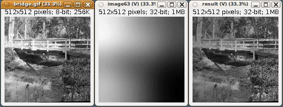
|
||||||
|
Extracting and manipulating image color channels: RGBA and HSB In the examples above we have already used the Red and Green functions. There's also Blue, Alpha, and a generic Channel that takes the channel index as argument--where red is 3, green is 2, blue is 1, and alpha is 4 (these numbers are related to the byte order in the 4-byte that makes up a 32-bit integer). The basic color operations have to do with extracting the color channel, for a particular color space (RGBA or HSB) The function RGBA takes from 1 to 4 arguments, and creates an RGBA image out of them. These arguments can be images, other functions, or numbers--for example, all pixels of a channel would have the value 255 (maximum intensity). |
from script.imglib.math import Compute, Subtract, Multiply
from script.imglib.color import Red, Blue, RGBA
from script.imglib.algorithm import Gauss, Dither
from ij import IJ

# Obtain a color image from the ImageJ samples
clown = ImgLib.wrap(IJ.openImage("https://imagej.nih.gov/ij/images/clown.jpg"))

# Example 1: compose a new image manipulating the color channels of the clown image:
img = RGBA(Gauss(Red(clown), 10), 40, Multiply(255, Dither(Blue(clown)))).asImage()

ImgLib.wrap(img).show()
| ||||||
|
In the second example, we extract the HSB channels from the clown image. To the Hue channel (which is expressed in the range [0, 1]), we add 0.5. We've shifted the hue around a bit.
|
from script.imglib.math import Compute, Add, Subtract
from script.imglib.color import HSB, Hue, Saturation, Brightness
from script.imglib import ImgLib
from ij import IJ

# Obtain an image
img = ImgLib.wrap(IJ.openImage("https://imagej.nih.gov/ij/images/clown.jpg"))

# Obtain a new clown, whose hue has been shifted by half
# with the same saturation and brightness of the original
bluey = Compute.inRGBA(HSB(Add(Hue(img), 0.5), Saturation(img), Brightness(img)))

ImgLib.wrap(bluey).show()
|
||||||
|
In the third example, we apply a gamma correction to an RGB confocal stack. To correct the gamma, we must first extract each color channel from the image, and then apply the gamma to each channel independently. In this example we use a gamma of 0.5 for every channel. Of course you could apply different gamma values to each channel, or apply it only to specific channels. Notice how we use asImage() instead of Compute.inRGBA. The result is the same; the former is syntactic sugar of the latter.
|
# Correct gamma
from script.imglib.math import Min, Max, Exp, Multiply, Divide, Log
from script.imglib.color import RGBA, Red, Green, Blue
from ij import IJ

gamma = 0.5
img = ImgLib.wrap(IJ.getImage())

def g(channel, gamma):
  """ Return a function that, when evaluated, computes the gamma
      of the given color channel.
      If 'i' was the pixel value, then this function would do:
      double v = Math.exp(Math.log(i/255.0) * gamma) * 255.0);
      if (v < 0) v = 0;
      if (v >255) v = 255;
  """
  return Min(255, Max(0, Multiply(Exp(Multiply(gamma, Log(Divide(channel, 255)))), 255)))

corrected = RGBA(g(Red(img), gamma), g(Green(img), gamma), g(Blue(img), gamma)).asImage()

ImgLib.wrap(corrected).show()
|
||||||
|
Find cells in an 3D image stack by Difference of Gaussian, count them, and show them in 3D as spheres. First we define the cell diameter that we are looking for (5 microns; measure it with a line ROI over the image) and the minimum voxel intensity that will care about (in this case, anything under a value of 40 will be ignored). And we load the image of interest: a 3-color channel image of the first instar Drosophila larval brain. Then we scale down the image to make it isotropic: so that voxels have the same dimensions in all axes. We run the DoGPeaks ("Difference of Gaussian Peaks") with a pair of appropriate sigmas: the scaled diameter of the cell, and half that. The peaks are each a float[] array that specifies its coordinate. With these, we create Point3f instances, which we transport back to calibrated image coordinates. Finally, we show in the 3D Viewer the peaks as spheres, and the image as a 3D volume. 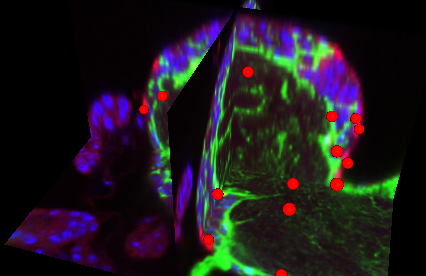
|
# Load an image of the Drosophila larval fly brain and segment
# the 5-micron diameter cells present in the red channel.

from script.imglib.analysis import DoGPeaks
from script.imglib.color import Red
from script.imglib.algorithm import Scale2D
from script.imglib.math import Compute
from script.imglib import ImgLib
from ij3d import Image3DUniverse
#from javax.vecmath import Color3f, Point3f # shadowed in Fiji by org.scijava.vecmath
from org.scijava.vecmath import Color3f, Point3f
from ij import IJ

cell_diameter = 5  # in microns
minPeak = 40 # The minimum intensity for a peak to be considered so.
imp = IJ.openImage("http://samples.fiji.sc/first-instar-brain.zip")

# Scale the X,Y axis down to isotropy with the Z axis
cal = imp.getCalibration()
scale2D = cal.pixelWidth / cal.pixelDepth
iso = Compute.inFloats(Scale2D(Red(ImgLib.wrap(imp)), scale2D))

# Find peaks by difference of Gaussian
sigma = (cell_diameter  / cal.pixelWidth) * scale2D
peaks = DoGPeaks(iso, sigma, sigma * 0.5, minPeak, 1)
print "Found", len(peaks), "peaks"

# Convert the peaks into points in calibrated image space
ps = []
for peak in peaks:
  p = Point3f(peak)
  p.scale(cal.pixelWidth * 1/scale2D)
  ps.append(p)

# Show the peaks as spheres in 3D, along with orthoslices:
univ = Image3DUniverse(512, 512)
univ.addIcospheres(ps, Color3f(1, 0, 0), 2, cell_diameter/2, "Cells").setLocked(True)
univ.addOrthoslice(imp).setLocked(True)
univ.show()
|
||||||
11. ImgLib2: writing generic, high-performance image processing programsFor a high-level introduction to ImgLib2, see:
|
|||||||
|
Views of an image, with ImgLib2 ImgLib2 is a powerful library with a number of key concepts for high-performance, memory-efficient image processing. One such concept is that of a view of an image. First, wrap a regular ImageJ ImagePlus into an ImgLib2 image, with the 'wrap' function in the ImageJFunctions namespace (AKA a static method), which we alias as IL for brevity using the as keyword in the import line. Then, we view the image as an infinite image, using the Views.extendZero function: beyond the boundaries of the image, return the value zero as the pixel value. An infinite image cannot be visualized in full. Therefore, we apply the Views.interval function to delimit it: in this example, to a "canvas" twice as large as before, with the image centered. Then, we wrap the ImgLib2 interval imgL into an ImageJ's ImagePlus (using a modified VirtualStack that reads directly from the imgL), and show it. Importantly, no pixel data was duplicated at any step. The Views concept enables us to define transformations to the image that are then concatenated and finally used to render the final image. And furthermore, thanks to ImgLib2's underlying dimension-independent, data source-independent, and image type-independent model, this code applies to any image of any type and dimensions: images, volumes, 4D series. ImgLib2 is a very powerful library. |
from ij import IJ
from net.imglib2.img.display.imagej import ImageJFunctions as IL
from net.imglib2.view import Views

# Load an image (of any dimensions) such as the clown sample image
imp = IJ.getImage()

# Convert to 8-bit if it isn't yet, using macros
IJ.run(imp, "8-bit", "")

# Access its pixel data from an ImgLib2 RandomAccessibleInterval
img = IL.wrapReal(imp)

# View as an infinite image, with a value of zero beyond the image edges
imgE = Views.extendZero(img)

# Limit the infinite image with an interval twice as large as the original,
# so that the original image remains at the center.
# It starts at minus half the image width, and ends at 1.5x the image width.
minC = [int(-0.5 * img.dimension(i)) for i in range(img.numDimensions())]
maxC = [int( 1.5 * img.dimension(i)) for i in range(img.numDimensions())]
imgL = Views.interval(imgE, minC, maxC)

# Visualize the enlarged canvas, so to speak
imp2 = IL.wrap(imgL, imp.getTitle() + " - enlarged canvas") # an ImagePlus
imp2.show()
|
||||||
|
There are multiple strategies for filling in the space beyond an image boundaries. Above, we used Views.extendZero, which trivally sets the "outside" to the pixel value zero. But there are several variants, including View.extendValue for arbitrary pixel values instead of zero; Views.extendMirrorSingle and Views.extendMirrorDouble for mirroring the pixel values relative to the nearest image border, and others. See Views for details and for more. In this example, we use Views.extendMirrorSingle and the effect is clear when we take an interval over it just like the one above: instead of the image surrounded by black space, we get mirror copies in every direction beyond the edges of the original image, which remains centered. The various extended views each have their purpose. Extending enables, for example, to avoid writing in special purpose code for e.g. algorithms that use a moving window around every pixel. The pixels on the border or near the border (depending on the size of the window) would need to be special-cased. Instead, with extended views, you can specify what data should be present beyond the border (a constant value, a mirror reflection of the image), and reduce enormously the complexity of your code. You could also use them like ROIs (regions of interest): obtain a View on a specific region of the image, and apply to it any code that runs on whole images. Views simplify programming for image processing a lot. |
img = ... # See above

# View mirroring the data beyond the edges
imgE = Views.extendMirrorSingle(img)
imgL = Views.interval(imgE, minC, maxC)

# Visualize the enlarged canvas, so to speak
imp2 = IL.wrap(imgL, imp.getTitle() + " - enlarged canvas") # an ImagePlus
imp2.show()
|
||||||
|
Create images To create an ImgLib2 image, we must choose a pixel type (e.g. UnsignedByteType for an 8-bit image) and a storage strategy (e.g. an in-memory array). The ArrayImgFactory is the straightforward yet verbose way to create an image, taking a type as argument and providing the create method that takes the dimensions as argument and returns a new ArrayImg: an image whose pixels are stored in a memory-resident java array, just like in a standard ImageJ ImagePlus. Reading the dimensions of an image gets tedious, so there's the Intervals.dimensionsAsLongArray method to read out the dimensions from any Interval; some examples of an Interval are RandomAccessibleInterval, IterableInterval, and a class that agglomerates both, Img. (Note all of these are interfaces. An ArrayImg implements Img.) And given that all images implement Interval--because they are defined within certain bounds for each dimension, otherwise they'd be infinite--, any instance of an "image" (in the broader sense of anything that implements Interval, because it also implements the Dimensions interface) can be used as the dimensions argument to the factory().create(...) call, as we do for creating img4 in the example. The advantage of using the img.factory().create() method is that the new image will be of the same kind and type as the original image. Which may or may not be what you want! To make a new image of the same kind (e.g. backed by java arrays) but of a different pixel type, use the img.factory().imgFactory(...) method that creates a new factory but for the newly provided pixel type. In the example, we give it a 16-bit type UnsignedShortType, and the same dimensions (by providing img as argument, using it as an interval from which to read the dimensions) to create imgShorts. |
from net.imglib2.img.array import ArrayImgFactory
from net.imglib2.type.numeric.integer import UnsignedByteType, UnsignedShortType
from net.imglib2.util import Intervals

# An 8-bit 256x256x256 volume
img = ArrayImgFactory(UnsignedByteType()).create([256, 256, 256])

# Another image of the same type and dimensions, but empty
img2 = img.factory().create([img.dimension(d) for d in xrange(img.numDimensions())])

# Same, but easier reading of the image dimensions
img3 = img.factory().create(Intervals.dimensionsAsLongArray(img))

# Same, but use an existing img as an Interval from which to read out the dimensions
img4 = img.factory().create(img)

# Now we change the type: same kind of image (ArrayImg) and same dimensions,
# but crucially a different pixel type (16-bit) via a new ImgFactory
factory16bit = img.factory().imgFactory(UnsignedShortType())
imgShorts = factory16bit.create(img) # empty 16-bit ArrayImg
|
||||||
|
For most use cases, ArrayImgs provide static methods to trivially create new ArrayImg instances. |
from net.imglib2.img.array import ArrayImgs

# An 8-bit 256x256x256 volume
img = ArrayImgs.unsignedBytes([256, 256, 256])
|
||||||
|
Imglib2 further provides additional kinds of images. The most interesting is the CellImg and its relatives the LazyCellImg and CachedCellImg. These images, among other features, enable overcoming the maximum 2GB length of a java array by partitioning the image into multiple cells (hence the name) in a grid. Each cell can have any number of dimensions, but all cells of the same image have the same. Also, they can have just one cell. And don't worry about the image dimensions not being an integer multiple of its cell dimensions; it'll just be less memory efficient. Cells can be of any dimensions: lines (in a 1-dimensional image), planes, cubes, etc. And that's a key feature of ImgLib2: images are dimension-, storage- and type-independent. Instead of images, think of them as data containers, or in mathematical terms, tensors. An example of this flexibility is the use of ImgLib2 data structures to represent DNA or RNA data, using the BasePairBitType, which stores ribonucleic bases (N, A, T, G, C, U) and a gap using 3 bits per entry. This type (not a pixel type!) doesn't have math methods; instead, it offers complement (e.g. given an A, return a T) and compareTo, and others. The BasePairCharType does the same but using 8 bits per entry, using a java char primitive type for each element of the ribonucleic sequence. Note that each cell is backed up by an "access" resource (where the pixels are stored) from the basictypeaccess package which can be backed by an array (e.g. ByteArray for a byte[]), but doesn't have to: you are free to implement your own classes that extend a particular access interface (e.g. ByteAccess) to provide data from the web, from a file, from a function, etc. This flexibility allows for data not existing in memory at all (the storage-independent aspect of ImgLib2) and being provided on demand, storing some of it temporarily in an in-memory cache--a functionality provided by the CachedCellImg (see an example using a CachedCellImg to represent a virtual stack with each image dynamically loaded from a file or retrieved from an in-memory cache). Think of these as a more powerful version of ImageJ's VirtualStack. |
from net.imglib2.img.cell import CellImgFactory
from net.imglib2.type.numeric.integer import UnsignedByteType

factory = CellImgFactory(UnsignedByteType(), [64, 64, 64])

# An 8-bit 256x256x256 volume, split into several 64x64x64 cubes
cell_img = factory.create([256, 256, 256])

grid = cell_img.getCellGrid()
print grid
CellGrid( dims = (256, 256, 256), cellDims = (64, 64, 64) )
|
||||||
|
Counting cells: difference of Gaussian peak detection with ImgLib2 First we load ImageJ's "embryos" example image, which is RGB, and convert it to 8-bit (16-bit or 32-bit would work just fine). Then we wrap it as an ImgLib2 image, and acquire a mirroring infinite view of the image which is suitable for computing Gaussians. The parameters of ImgLib2's Difference of Gaussian detection (DogDetection) are relatively straightforward. The key parameters are the sigmaLarger and sigmaSmaller, which define the sigmas of the two Gaussians that will be subtracted one from the other. The minPeakValue acts as a filter for noisy detections. The calibration would be useful in e.g. an LSM 3D volume where the Z axis has typically a lower resolution than the X and Y axes. For visual validation, we read out the detected peaks as a PointRoi that we set on the imp, the original ImagePlus with the embryos (see image below with a PointRoi point on each embryo). Then, we set out to measure a small interval around each detected peak (each embryo). For this, we use the sigmaSmaller, which is half of the radius of an embryo (determined empirically by using a line ROI over embryos and pushing 'm' to measure them), so that we define a 2d box around the peak, with a side twice that of sigmaSmaller plus one. Ideally, one would use a circular ROI by using a HyperSphere, but a square ROI as obtained with a View.interval will more than suffice here. Picking and measuring areas with Views.interval To sum the pixel intensity values within the interval, we use Views.flatIterable on the interval, which provides a view that can be serially iterated over the interval. Otherwise, the interval, which is a RandomAccessibleInterval, would yield its pixel values only if we gave it each pixel coordinate to be measured. Then, we iterate each small view, obtaining a t (a Type) instance for every pixel, which in ImgLib2 is one of the key design features that enables so much indirection without sacrificing performance. To the t Type, which is a subclass of NumericType, we ask it to yield an integer with t.getInteger(). Python's built-in sum function adds up all the values of the generator (no list is created). Listing measurements with a Results Table Finally, the peak X,Y coordinates and the sum of pixel values within the interval are added to an ImageJ ResultsTable.
|
from ij import IJ
from ij.gui import PointRoi
from ij.measure import ResultsTable
from net.imglib2.img.display.imagej import ImageJFunctions as IL
from net.imglib2.view import Views
from net.imglib2.algorithm.dog import DogDetection
from jarray import zeros

# Load a greyscale single-channel image: the "Embryos" sample image
imp = IJ.openImage("https://imagej.nih.gov/ij/images/embryos.jpg")
# Convert it to 8-bit
IJ.run(imp, "8-bit", "")

# Access its pixel data from an ImgLib2 data structure: a RandomAccessibleInterval
img = IL.wrapReal(imp)

# View as an infinite image, mirrored at the edges which is ideal for Gaussians
imgE = Views.extendMirrorSingle(img)

# Parameters for a Difference of Gaussian to detect embryo positions
calibration = [1.0 for i in range(img.numDimensions())] # no calibration: identity
sigmaSmaller = 15 # in pixels: a quarter of the radius of an embryo
sigmaLarger = 30  # pixels: half the radius of an embryo
extremaType = DogDetection.ExtremaType.MAXIMA
minPeakValue = 10
normalizedMinPeakValue = False

# In the differece of gaussian peak detection, the img acts as the interval
# within which to look for peaks. The processing is done on the infinite imgE.
dog = DogDetection(imgE, img, calibration, sigmaSmaller, sigmaLarger,
  extremaType, minPeakValue, normalizedMinPeakValue)

peaks = dog.getPeaks()

# Create a PointRoi from the DoG peaks, for visualization
roi = PointRoi(0, 0)
# A temporary array of integers, one per dimension the image has
p = zeros(img.numDimensions(), 'i')
# Load every peak as a point in the PointRoi
for peak in peaks:
  # Read peak coordinates into an array of integers
  peak.localize(p)
  roi.addPoint(imp, p[0], p[1])

imp.setRoi(roi)

# Now, iterate each peak, defining a small interval centered at each peak,
# and measure the sum of total pixel intensity,
# and display the results in an ImageJ ResultTable.
table = ResultsTable()

for peak in peaks:
  # Read peak coordinates into an array of integers
  peak.localize(p)
  # Define limits of the interval around the peak:
  # (sigmaSmaller is half the radius of the embryo)
  minC = [p[i] - sigmaSmaller for i in range(img.numDimensions())]
  maxC = [p[i] + sigmaSmaller for i in range(img.numDimensions())]
  # View the interval around the peak, as a flat iterable (like an array)
  fov = Views.interval(img, minC, maxC)
  # Compute sum of pixel intensity values of the interval
  # (The t is the Type that mediates access to the pixels, via its get* methods)
  s = sum(t.getInteger() for t in fov)
  # Add to results table
  table.incrementCounter()
  table.addValue("x", p[0])
  table.addValue("y", p[1])
  table.addValue("sum", s)

table.show("Embryo intensities at peaks")

# Also show the image with the PointRoi on it:
imp.show()
|
||||||
|
Saving measurements into a CSV file, and reading them out as a PointRoi Let's learn how to save the data to a CSV file. There are multiple ways to do so. In the Results Table window, choose "File - Save...", which will save the table data in CSV format. Doesn't get any easier than this! In the absence of a Results Table, we can use python's built-in csv library. First, we define two functions to provide the data (peakData and the helper function centerAt), so that (for simplicity and clarity) we separate getting the peak data from writing the CSV. To get the peak data, we define the function peakData that does the same as was done above in a for loop: localize the peak (which writes its coordinates into the float array p) and then sum the pixels around the peak using an interval view. The helper function centerAt returns two copied arrays with the two arrays (minC, maxC) that delimit the region of interest around the peak translated to the peak. Then, we write the CSV file one row at a time. We open the file within python's with statement, which ensures that, even if an error was to come up, the file handle will be closed, properly releasing system resources. The csv.writer function returns an object w onto which we call writerow for every peak. Notice the arguments provided to csv.writer, defining the delimiter (a comma, a space, a tab...), the quote character (for strings), and what to quote (everything that is not a number). The first row is the header, containing the titles of each column in the CSV file. Then each data row is written by providing writerow with the list of column entries to write: x, y and s, which is the sum of pixel values within the interval around x,y. For completeness, I am showing here how to read the CSV file back into, in this example, a PointRoi, using the complementary function csv.reader. Note that numeric values are read in as strings, and must be transformed into floating-point numbers using the built-in function float.
|
from __future__ import with_statement
# IMPORTANT: imports from __future__ must go at the top of the file.

#
# ... same code as above here to obtain the peaks
#

from operator import add
import csv

# The minumum and maximum coordinates, for each image dimension,
# defining an interval within which pixel values will be summed.
minC = [-sigmaSmaller for i in xrange(img.numDimensions())]
maxC = [ sigmaSmaller for i in xrange(img.numDimensions())]

def centerAt(p, minC, maxC):
  """ Translate the minC, maxC coordinate bounds to the peak. """
  return map(add, p, minC), map(add, p, maxC)

def peakData(peaks, p, minC, maxC):
  """ A generator function that returns all peaks and their pixel sum,
      one at a time. """
  for peak in peaks:
    peak.localize(p)
    minCoords, maxCoords = centerAt(p, minC, maxC)
    fov = Views.interval(img, minCoords, maxCoords)
    s = sum(t.getInteger() for t in fov)
    yield p, s

# Save as CSV file
with open('/tmp/peaks.csv', 'wb') as csvfile:
  w = csv.writer(csvfile, delimiter=',', quotechar="\"",
                 quoting=csv.QUOTE_NONNUMERIC)
  w.writerow(['x', 'y', 'sum'])
  for p, s in peakData(peaks, p, minC, maxC):
    w.writerow([p[0], p[1], s])

# Read the CSV file into an ROI
roi = PointRoi(0, 0)
with open('/tmp/peaks.csv', 'r') as csvfile:
  reader = csv.reader(csvfile, delimiter=',', quotechar="\"")
  header = reader.next() # advance reader by one line
  for x, y, s in reader:
    roi.addPoint(imp, float(x), float(y))

imp.show()
imp.setRoi(roi)
|
||||||
|
Generative image: simulating embryo segmentation Here, I am showing how to express images whose underlying data is not the typical array of pixels, but rather, each pixel value is chosen as a function of the spatial coordinate. The underlying pixel data is just the function. In this example, a white pixel is returned when the pixel falls within a radius of the detected embryo, and a black pixel otherwise, for the background. You may ask yourself what is the point of this simulated object segmentation. It is merely to illustrate how these function-based images can be created. Practical uses will come later. If you want a real segmentation of the area of these embryos, see Fiji/ImageJ's "Analyze - Analyze Particles...", or the machine-learning based Trainable WeKa Segmentation and SIOX simple interactive object extraction plugins. First, we detect embryos using the Difference of Gaussian approach used above, with the DogDetection class. From this, we obtain the centers of all detected embryos, in floating-point coordinates. Second, we define a value for the inside of the embryo (white), and another for the outside (black, the background). Then we specify the radius that we want to paint with the inside value around the center coordinate of every detected embryo. And crucially, we construct a KDTree, which is a data structure for fast spatial queries of coordinates. Here we use the kdtree to swiftly find, for every pixel in the final image, the nearest embryo center point. Then, we define our "image". In quotes, because it is not an image. What we define is a method to obtain pixel values at arbitrary spatial coordinates, returning either inside (white) or outside (black) depending on the position in space for which we request a value. To this end, we define a new class Circles that is a RealRandomAccess, and, to avoid having to implement all the necessary methods of the RealRandomAccess interface, we extend the RealPoint class too, because it already implements pretty much everything we need except the critical get method from the Sampler interface. In other words, the only practical difference between a RealPoint and a RealRandomAccess is that the latter also implements the Sampler interface for requesting values. The search is implemented using a NearestNeighborSearchOnKDTree, which does exactly what it says, and offers a stateful search.search. method: first we invoke the search (at the implicit current spatial coordinate of the RealRandomAccess parts of the Circles class), and then we ask for the distance from the current coordinate to the nearest one that was found in the search. On the basis of the result--comparing with the radius--either the inside or the outside is returned. All that remains now is using the Circles RealRandomAccess as the data provider for a RealRandomAccessible that we name CircleData, which is still in real coordinates and unbounded. So we view it in a rasterized way, to be able to iterate it with integer coordinates--like the pixels of an image--, and define its bounds to be those of the original image img containing the embryos (that is, img here can be used because it implements Interval and happens to have exactly the dimensions we want). The "pixels" never exist in memory until they are written to the final image that is visualized. Voilà. |
from ij import IJ
from net.imglib2.view import Views
from net.imglib2.algorithm.dog import DogDetection
from net.imglib2 import KDTree, RealPoint, RealRandomAccess, RealRandomAccessible
from net.imglib2.neighborsearch import NearestNeighborSearchOnKDTree
from net.imglib2.img.display.imagej import ImageJFunctions as IL
from net.imglib2.type.numeric.integer import UnsignedByteType
from java.util import AbstractList

# The difference of Gaussian calculation, same as above (compressed)
# (or, paste this script under the script above where 'dog' is defined)
imp = IJ.openImage("https://imagej.nih.gov/ij/images/embryos.jpg")
IJ.run(imp, "8-bit", "")
img = IL.wrapReal(imp)
imgE = Views.extendMirrorSingle(img)
dog = DogDetection(imgE, img, [1.0, 1.0], 15.0, 30.0,
  DogDetection.ExtremaType.MAXIMA, 10, False)

# The spatial coordinates for the centers of all detected embryos
centers = dog.getSubpixelPeaks() # in floating-point precision

# A value for the inside of an embryo: white, in 8-bit
inside = UnsignedByteType(255)

# A value for the outside (the background): black, in 8-bit
outside = UnsignedByteType(0)

# The radius of a simulated embryo, same as sigmaLarger was above
radius = 30 # or = sigmaLarger

# KDTree: a data structure for fast lookup of spatial coordinates
kdtree = KDTree([inside] * len(centers), centers)

# The definition of circles (or spheres, or hyperspheres) in space
class Circles(RealPoint, RealRandomAccess):
  def __init__(self, n_dimensions, kdtree, radius, inside, outside):
    super(RealPoint, self).__init__(n_dimensions)
    self.search = NearestNeighborSearchOnKDTree(kdtree)
    self.radius = radius
    self.radius_squared = radius * radius
    self.inside = inside
    self.outside = outside
  def copyRealRandomAccess(self):
    return Circles(self.numDimensions(), self.kdtree, self.radius,
                   self.inside, self.outside)
  def get(self):
    self.search.search(self)
    if self.search.getSquareDistance() < self.radius_squared:
      return self.inside
    return self.outside

# The RealRandomAccessible that wraps the Circles in 2D space, unbounded
# NOTE: partial implementation, unneeded methods were left unimplemented
class CircleData(RealRandomAccessible):
  def realRandomAccess(self):
    return Circles(2, kdtree, radius, inside, outside)
  def numDimensions(self):
    return 2

# An unbounded view of the Circles that can be iterated in a grid, with integers
raster = Views.raster(CircleData())

# A bounded view of the raster, within the bounds of the original 'img'
# I.e. 'img' here is used as the Interval within which the CircleData is defined
circles = Views.interval(raster, img)

IL.wrap(circles, "Circles").show()
|
||||||
|
Transform an image using ImgLib2. In this example, we will use ImgLib2's RealViews namespace to transform images with affine transforms: translate, rotate, scale, shear. Let's introduce the concept of a View in ImgLib2: it's like a shallow copy, possibly transformed. Meaning, the underlying pixel array is not duplicated, with merely a transformation of some sort being applied to the pixels on the fly as these are requested. Views can be concatenated. Here we use:
While the reasons that led to split the functionality into two separate namespaces (the Views and the RealViews) don't matter, the basic heuristic when looking up for a View method is that we'll use Views when the interval is defined (that is, the image data is known to exist within a specific range between 0 and width, height, depth, etc., which is almost always), and we'll use RealViews when the interval is not defined and pixels can be retrieved with real numbers, that is, floating point numbers (such as when applying affine transforms or performing interpolations). In the end, we call ImageJFunctions.wrap again to visualize the transformed image as a regular ImageJ's ImagePlus containing a VirtualStack whose pixel source is the scaled up View, whose pixel source, in turn, is the original ImagePlus. No data has been duplicated at any step! |
from net.imglib2.realtransform import RealViews as RV
from net.imglib2.img.display.imagej import ImageJFunctions as IL
from net.imglib2.realtransform import Scale
from net.imglib2.view import Views
from net.imglib2.interpolation.randomaccess import NLinearInterpolatorFactory
from ij import IJ

# Load an image (of any dimensions)
imp = IJ.getImage()

# Access its pixel data as an ImgLib2 RandomAccessibleInterval
img = IL.wrapReal(imp)

# View as an infinite image, with a value of zero beyond the image edges
imgE = Views.extendZero(img)

# View the pixel data as a RealRandomAccessible
# (that is, accessible with sub-pixel precision)
# by using an interpolator
imgR = Views.interpolate(imgE, NLinearInterpolatorFactory())

# Obtain a view of the 2D image twice as big
s = [2.0 for d in range(img.numDimensions())] # as many 2.0 as image dimensions
bigger = RV.transform(imgR, Scale(s))

# Define the interval we want to see: the original image, enlarged by 2X
# E.g. from 0 to 2*width, from 0 to 2*height, etc. for every dimension
minC = [0 for d in range(img.numDimensions())]
maxC = [int(img.dimension(i) * scale) for i, scale in enumerate(s)]
imgI = Views.interval(bigger, minC, maxC)

# Visualize the bigger view
imp2x = IL.wrap(imgI, imp.getTitle() + " - 2X") # an ImagePlus
imp2x.show()
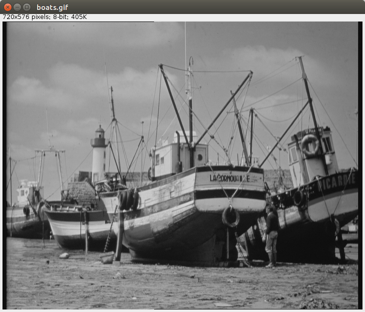 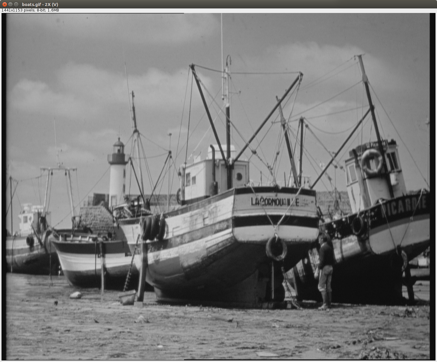
|
||||||
|
At any time, use e.g. print type(imgR) to see the class of e.g. the object imgR. Then, either look it up in the ImgLib2's github repositories or in Google, or perhaps sufficiently, use print dir(imgR) to list all its accessible methods.
|
print type(imgR)
print dir(imgR)
<type 'net.imglib2.interpolation.Interpolant'>

['__class__', '__copy__', '__deepcopy__', '__delattr__', '__doc__',
'__ensure_finalizer__', '__eq__', '__format__', '__getattribute__',
'__hash__', '__init__', '__ne__', '__new__', '__reduce__', '__reduce_ex__',
'__repr__', '__setattr__', '__str__', '__subclasshook__', '__unicode__',
'class', 'equals', 'getClass', 'getInterpolatorFactory', 'getSource',
'hashCode', 'interpolatorFactory', 'notify', 'notifyAll', 'numDimensions',
'realRandomAccess', 'source', 'toString', 'wait']
|
||||||
|
The resulting ImagePlus can be saved using ImageJ's FileSaver methods, just like any other ImageJ image. |
from ij.io import FileSaver

FileSaver(imp2x).saveAsPng("/path/to/boats-2x.png")
|
||||||
|
Intermezzo: iterate n-dimensional image corners with destructuring and combinatoric generators In the example below, we'll needed to compute and iterate over the coordinates of all corners of a 3-dimensional volume, but we would like to write the code in a way that allows us to do the same for images with any number of dimensions. It's also a compact way to write code; a way by which we specify what we want rather than the explicity details. Let's unpack the code here for clarity. First, the explicit code. The list corners contains the coordinates for all 8 corners of a 3-dimensional volume. |
width = 512
height = 512
depth = 512
maxX = width -1
maxY = height -1
maxZ = depth - 1

corners = [[0, 0, 0],
           [maxX, 0, 0],
           [0, maxY, 0],
           [maxX, maxY, 0],
           [0, 0, maxZ],
           [maxX, 0, maxZ],
           [0, maxY, maxZ],
           [maxX, maxY, maxZ]]
|
||||||
|
Notice there's lots of repetition in the manually specified corners list. Clearly, there's a pattern: each coordinate (X, Y, Z) of each corner can only ever take one of two values: either 0 or the maximum value for that dimension. Therefore, what we want is a list of these pairs of possible values, and then generate the corner coordinates from it. We define the pairs of values for each dimension in a dictionary (a list of lists would also do), and then run a triple loop to generate all possible combinations, generating the coordinates for the 8 corners. |
values = {'x': [0, maxX],
          'y': [0, maxY],
          'z': [0, maxZ]}

corners = []

for vZ in values['z']:
  for vY in values['y']:
    for vX in values['x']:
      corners.append([vX, vY, vZ])

from pprint import pprint
pprint(corners)
[[0, 0, 0],
 [511, 0, 0],
 [0, 511, 0],
 [511, 511, 0],
 [0, 0, 511],
 [511, 0, 511],
 [0, 511, 511],
 [511, 511, 511]]
|
||||||
|
That was much better, and also it's harder to introduce an error. But if we were to remove further repetitive code, then we would remove the dimension constraint: we could generate lists of corner coordinates for 2-dimensional, 3-dimensional, 4-dimensional images, or for any number of dimensions. The first repetition is the pairs of values that each coordinate can take for each dimension. Automating these is easy: for each pair, the first is a zero always, and the second is the size of the dimension minus one, or the maximum value. Each ImgLib2 image is an Interval, which, by definition, has a minimum and a maximum coordinate defined for each of its dimensions, in addition to a size of each dimension. We use list comprehension to populate the values list with the pairs. Note that here we assume that the interval starts at zero, but it doesn't have to (hence the Views.zeroMin method to pretend that it does). In such cases you'd use img.min(d) instead of hard-coding a zero. Now we must address the loop: for an n-dimensional image, we can't hardcode the number of nested loops because we don't know them a priori. Therefore, we resort to combinatoric generators from the itertools package package. In particular we will use product, which takes an arbitrary number of sequences as arguments and does exactly what we want: the cartesian product, generating all possible combinations. For a truly n-dimensional cartesian product, we have to not manually specify the pairs of values provided to product (that would defeat the purpose), but instead use python's asterisk notation for unpacking the elements of a list as the arguments that a function receives. With that, our code is now generic to any number of dimensions. The printed corners are exactly the same as before, but in a different order (Z is the fastest coordinate instead of the X, which is now the slower), and each number is a long (hence the 'L') rather than an integer, since ImgLib2 uses longs for its dimensions. Note that product creates a generator. To reify it--to make it exist--we tell a list to populate itself from the content of the generator.
|
from net.imglib2.img.array import ArrayImgs
from net.imglib2.util import Intervals
from itertools import product

img = ArrayImgs.unsignedBytes([512, 512, 512]) # a 3D image

values = [[0, img.dimension(d) - 1] for d in xrange(img.numDimensions())]

# Or what is the same, but shorter:
# (the max integer coordinate is img.dimension(d) -1)
# (the min interger coordinate is often zero, but doesn't have to be)
values = [[img.min(d), img.max(d)] for d in xrange(img.numDimensions())]

# Or the same again, even shorter, assuming the min is always zero:
values = [[0, v] for v in Intervals.maxAsLongArray(img)]

# Specify a generator for all 8 corners of a 3D volume
corners_gen = product(values[0], values[1], values[2])

# Now with a truly n-dimensional loop:
# the asterisk unpacks the elements of the values list, providing
# each as argument to the product function
corners_gen = product(*values)

# Create the list of corners by populating a list from the generator
# (only needed if you want the list to persist; otherwise simply consume
# the generator the one time that is needed.)
corners = list(corners_gen)

for corner in corners:
  print corner
(0, 0, 0)
(0, 0, 511L)
(0, 511L, 0)
(0, 511L, 511L)
(511L, 0, 0)
(511L, 0, 511L)
(511L, 511L, 0)
(511L, 511L, 511L)
|
||||||
|
To better explain how the asterisk list unpacking works, consider this example. |
numbers = [0, 1, 2]

# Individual assignment
zero = numbers[0]
one = numbers[1]
two = numbers[2]

# Or what is the same: destructuring assignment onto multiple variables
zero, one, two = numbers

def sum(first, second, third):
  return first + second + third

total = sum(numbers[0], numbers[1], numbers[2])

# Or what is the same: destructuring assigment onto function arguments
total = sum(*numbers)
|
||||||
|
In a loop, you can also destructure. Consider this example, where a list of pairs (generated with the built-in zip command) is then iterated first by pair, and then by the elements of the pair. |
names = ["zero", "one", "two"]
numbers = [0, 1, 2]

pairs = zip(names, numbers)

for pair in pairs:
  print pair

# Or what is the same, but with more control:
for name, number in pairs:
  print name + ": " + str(number)
('zero', 0)
('one', 1)
('two', 2)

zero: 0
one: 1
two: 2
|
||||||
|
When looping over two lists, with one list having e.g. pairs as elements, then the destructuring of the elements of the pairs has to go in parentheses. So for each iteration of the loop there is the pair, that comes from the data_pairs, and is destructured into (fruit, weight), and then there is the index from the other list (actually the ordinal number generator built-in function xrange). Instead of manually using xrange, here I introduce enumerate, a built-in function that wraps a sequence and returns the equivalent of a zip of xrange and the sequence; in other words, enumerate takes a sequence and generates a sequence of pairs, with the first element being an index and the second the element of the sequence provided as argument. It's a more readable way to obtain (in a way, expose) the index of each step in the loop. For printing, notice we use the string formatting nomenclature, where, inside the string, the percent signs plus letters will be replaced by the corresponding variable (by order) in the list that follows the string after the outer percent sign. The letters following the percent sign inside the string are used to format a variable's content according to its data type, which the programmer knows but python, shockingly, doesn't. For a string (i.e. text within parentheses) use %s, for an integer number use %i, for a floating-point number use %f, which optionally can be made to specify how many decimal points to print, e.g. %.2f would print only two decimals.
|
fruit = ["apple", "orange", "pear"]
weight = [0.2, 0.4, 0.3]

data_pairs = zip(fruit, weight)

for (fruit, weight), index in zip(data_pairs, xrange(len(data_pairs))):
  print "entry %i has %s with weight %0.2f" % (index+1, fruit, weight)


# Or what is the same: use the enumerate built-in loop indexing function
for index, (fruit, weight) in enumerate(data_pairs):
  print "entry %i has %s with weight %0.2f" % (index+1, fruit, weight)
entry 1 has apple with weight 0.20
entry 2 has orange with weight 0.40
entry 3 has pear with weight 0.30
|
||||||
|
Rotating image volumes with ImgLib2. Now we continue with a rotation around the Z axis (rotation in XY) by 30 degrees. Remember, this code applies to images of any number of dimensions: would work equally well as is for the boats image example above. For the purpose of rotating a 3D image around the Z axis, we specifically use an AffineTransform3D, which offers the method rotate, requiring as arguments the axis of rotation (0 is X, 1 is Y, 2 is Z) and the angle in radians. (For an entirely n-dimensional image, use AffineTransform, which takes a Jama.Matrix as argument for its constructor.) By default, any rotation would use as center the 0, 0, 0 coordinate. We want to rotate relative to the center of the image instead. So first we define toCenter, a transformation that specifies a negative translation by as much as the center of the image in the XY plane. We fold this into the rotation with preConcatenate prior to invoking rotate. After rotate, we 'undo' the negative translation by specifying another translation, to the center of the XY plane, with another call to preConcatenate, this time with the inverse of the toCenter translation. Notice the rotated image is merely a transformed view (via ImgLib2's RealViews.transform) of a non-linear interpolated view of an extended zero-padded (think infinite) view of our original image. To render it, we must define the interval within which we want to observe the data. There are two obvious options: first, imgRot2d shows the result within the same interval as the original img, which will crop its corners, as the latter now fall outside of the field of view. Second, we can compute where the corners of the volume are now, use them to find out the minimum and maximum coordinates of the now rotated volume, and define an Interval with them, via Views.interval, shown as imgRot2dF . (Eventually there will be an util method in imglib2 to trivially compute the interval of an affine transformed image.) Notice that the code for computing the new minimally enclosing interval makes heavy use of perhaps lesser know python features (see above for a gentle introduction). For example, list unpacking with the asterisk, so that a function is invoked with the contents of a list populating each of its necessary arguments, rather than providing the function with a single argument (the list). As well as repeat (which creates a generator, so that from a single value as argument, it returns an infinite sequence) and product (to convert e.g. three pairs like [0, 512], [0, 512], [0, 512] into a sequence of all possible triplets, each element of each triplet being from one of the three pairs provided) that spares us from writing tedious and repetitive nested loops to accomplish the same. Both of these functions are from the itertools package, which offers additional, useful functions such as chain.from_iterable (to flatten a list of lists into a single list), other functions to generate combinations and permutations from the elements of a sequence or list, and, among several others, 'i' versions of the built-in zip and slice functions, with izip and islice returning generators rather than lists, for more memory-friendly code if the generators are consumed on the fly rather than their contents copied into short-lived lists. An additional new python feature shown here is list element unpacking, known as destructuring assignment, in a for loop inside a list comprehension (line 85): the sequence of pairs in bounds is looped over as (vmin, vmax), in other words accessing the values inside each pair directly rather than the containing pair itself (a tuple); so the loop has three variables: vmin, vmax and v originating from only two lists (bounds and transformed), with the first list containing pairs (that get unpacked into the numeric values vmin, vmax) and the second list containing individual numeric values (v). This approach eliminates the need for local variables and makes for more compact code, while maintaining readibility. (What can be opaque here is why we loop over a generator of corners at all: to keep the code flexible regarding the number of dimensions of the image, instead of hard-coding them.) Then we view the rotated image as an ImagePlus that wraps a VirtualStack just like above. In this particular example the effect is not very visible because the MRI stack of a human head has black corners. To reveal the issue of cropped corners, I draw a white line along the borders beforehand by pushing 'a' to select all with a rectangular ROI, then choosing white color for the foreground color, and then pushing 'd' to draw it, confirming the dialog to draw in every section.
|
import sys
from itertools import product, repeat
from net.imglib2.realtransform import RealViews as RV
from net.imglib2.realtransform import AffineTransform3D
from net.imglib2.img.display.imagej import ImageJFunctions as IL
from ij import IJ
from net.imglib2.view import Views
from net.imglib2.interpolation.randomaccess import NLinearInterpolatorFactory
from net.imglib2.util import Intervals
from math import radians, floor, ceil
from jarray import zeros


# Load an image (of any dimensions)
imp = IJ.getImage()

# Access its pixel data as an ImgLib2 RandomAccessibleInterval
img = IL.wrapReal(imp)

# View as an infinite image, with value zero beyond the image edges
imgE = Views.extendZero(img)

# View the pixel data as a RealRandomAccessible
# (that is, accessible with sub-pixel precision)
# by using an interpolator
imgR = Views.interpolate(imgE, NLinearInterpolatorFactory())

# Define a rotation by +30 degrees relative to the image center in the XY axes
angle = radians(30)
toCenter = AffineTransform3D()
cx = img.dimension(0) / 2.0  # X axis
cy = img.dimension(1) / 2.0  # Y axis
toCenter.setTranslation(-cx, -cy, 0.0) # no translation in the Z axis
rotation = AffineTransform3D()
# Step 1: place origin of rotation at the center of the image
rotation.preConcatenate(toCenter)
# Step 2: rotate around the Z axis
rotation.rotate(2, angle)  # 2 is the Z axis, or 3rd dimension
# Step 3: undo translation to the center
rotation.preConcatenate(toCenter.inverse()) # undo translation to the center

# Define a rotated view of the image
rotated = RV.transform(imgR, rotation)

# View the image rotated, without enlarging the canvas
# so we define the interval (here, the field of view of an otherwise infinite
# image) as the original image dimensions by using "img", which in itself is
# an Interval.
imgRot2d = IL.wrap(Views.interval(rotated, img), imp.getTitle() + " - rot2d")
imgRot2d.show()

# View the image rotated, enlarging the interval to fit it.
# (This is akin to enlarging the canvas.)

# We define each corner of the nth-dimensional volume as a combination,
# namely the 'product' (think nested loop) of the pairs of possible values
# that each dimension can take in every corner coordinate, zipping each
# with the value zero (hence the repeat(0) to provide as many as necessary),
# and then unpacking the list of pairs by using the * in front of 'zip'
# so that 'product' receives the pairs as arguments rather than a list of pairs.
# Because here 'product' receives 3 pairs, it outputs a sequence of triplets,
# one for each corner of the volume.
# Then we apply the transform to each corner, reading out the transformed
# coordinates by using the 'transformed' float array.

# We compute the bounds by, for every corner, checking if the floor of each
# dimension of a corner coordinate is smaller than the previously found
# minimum value, and by checking if the ceil of each corner coordinate is
# larger than the previously found value, packing the new pair of minimum
# and maximum values into the list of pairs that is 'bounds'.

# Notice the min coordinates can have negative values, as the rotated image
# has pixels now somewhere to the left and up from the top-left 0,0,0 origin
# of coordinates. That's why we use Views.zeroMin, to ensure that downstream
# uses of the transformed image see it as fitting within bounds that start
# at 0,0,0.

bounds = repeat((sys.maxint, 0)) # initial upper- and lower-bound values
                                 # for min, max to compare against
transformed = zeros(3, 'f')

for corner in product(*zip(repeat(0), Intervals.maxAsLongArray(img))):
  rotation.apply(corner, transformed)
  bounds = [(min(vmin, int(floor(v))), max(vmax, int(ceil(v))))
            for (vmin, vmax), v in zip(bounds, transformed)]

minC, maxC = map(list, zip(*bounds)) # transpose list of 3 pairs
                                     # into 2 list of 3 values
imgRot2dFit = IL.wrap(Views.zeroMin(Views.interval(rotated, minC, maxC)),
  imp.getTitle() + " - rot2dFit")
imgRot2dFit.show()
|
||||||
|
To read out the values of the transformation matrix that specifies the rotation, print it: it's an array containing the concatenated rows of the matrix. Or pretty-print it with pprint, which requires turning the arrays into lists for nicer printing. Given the desired 30 degree rotation, the "scale" part (the diagonal) becomes the cosine of 30 degrees (sqrt(3)/2 = 0.866), and the "shear" part (the second column of the first row, and the first column of the second row) becomes the sine of 30 degrees (0.5) with the appropriate sign (to the "left" for X, hence negative; and to the "right" for Y, hence positive). The third column contains the translation values corresponding to a rotation specified relative to the center of the image. While you could always write in the matrix by hand, it is better to use libraries like, for 2D, the java.awt.geom.AffineTransform and its methods such as getRotateInstance. For 3D rotations and affine transformations in general, use e.g. javax.media.j3d.Transform3D and e.g. its method rotZ, which sets the transform to mean a rotation in the Z axis, just like we did in this example with imglib2's AffineTransform3D.rotate. Or just use imglib2, like we did here, which is built explicitly for the purpose.
|
from pprint import pprint

matrix = rotation.getRowPackedCopy()
print matrix
pprint([list(matrix[i:i+4]) for i in xrange(0, 12, 4)))])
array([D, [array('d', [0.8660254037844387, -0.49999999999999994, 0.0,
68.95963744804719]), array('d', [0.49999999999999994, 0.8660254037844387,
0.0, -31.360870627641567]), array('d', [0.0, 0.0, 1.0, 0.0])])

[[0.8660254037844387,  -0.49999999999999994, 0.0,  68.95963744804719],
 [0.49999999999999994,  0.8660254037844387,  0.0, -31.360870627641567],
 [0.0,                  0.0,                 1.0,  0.0]]
|
||||||
|
Processing RGB and ARGB images with ImgLib2. An ARGB image is a hack: the four color channels have been stored each in one of the 4 bytes of a 32-bit integer. Processing directly the pixel array, made of integers, makes no sense at all. Prior to any processing, color channels must be separated. For reference, the alpha channel is in the upper byte (index 0), the red in the 2nd (index 1), the green in the 3rd (index 2) and blue in the lowest byte, the 4th (index 3). In ImgLib2, rather than copying a color channel into a new image with a new array of bytes, we acquire a View of its channels: by using the Converters functions, optionally together with the Views.hyperSlice functionality. First, we load an RGB or ARGB image and wrap it as an ImgLib2 object (despite what IL.wrapRGBA seems to imply, the alpha channel is still at index 0). If the ImagePlus is not backed by a ColorProcessor, it will throw an error. Then we invoke one of the several functions in the Converters namespace that handles ARGB images. Here, we use Converters.argbChannels, which delivers a view of the ARGB image as a stack of 4 images, one per channel. The channels image is equivalent to ImageJ's CompositeImage, in that each channel can be processed independently. To read out a single channel, e.g. the red channel (index 1), we could use Converters.argbChannel(img, 1). Or, as we illustrate here, use Views.hyperSlice: a function to reduce the dimensionally of an image, in this case by fixing the last dimension (the channels) to always be the red channel (at index 1). Of course, this code runs on 2D images (e.g. the leaf) or 3D images (e.g. the Drosophila larval brain LSM stack), or 4D images, or images of any dimensions. |
from net.imglib2.converter import Converters
from net.imglib2.view import Views
from net.imglib2.img.display.imagej import ImageJFunctions as IL
from ij import IJ

# # Load an RGB or ARGB image
imp = IJ.getImage()

# Access its pixel data from an ImgLib2 data structure:
# a RandomAccessibleInterval<ARGBType>
img = IL.wrapRGBA(imp)

# Convert an ARGB image to a stack of 4 channels:
#   a RandomAccessibleInterval<UnsignedByte>
# with one more dimension that before.
# The order of channels in the stack can be changed by changing their indices.
channels = Converters.argbChannels(img, [0, 1, 2, 3])

# Equivalent to ImageJ's CompositeImage: channels are separate
impChannels = IL.wrap(channels, imp.getTitle() + " channels")
impChannels.show()

# Read out a single channel directly
red = Converters.argbChannel(img, 1)

# Alternatively, pick a view of the red channel in the channels stack.
# Takes the last dimension, which are the channels,
# and fixes it to just one: that of the red channel (1) in the stack.
red = Views.hyperSlice(channels, channels.numDimensions() -1, 1)

impRed = IL.wrap(red, imp.getTitle() + " red channel")
impRed.show()
|
||||||
|
Analysis of 4D volumes with ImgLib2: GCaMP imaging data In neuroscience, we can observe the activity of neurons in a circuit by expressing, for example, a calcium sensor in every neuron of interest, generally using viruses as delivery vectors for mammals, birds and reptiles, or genetic constructs for the fruit fly Drosophila, the nematode C. elegans and zebrafish. From the many options available, we'll use data here from those called genetically encoded calcium indicators (GECI), the most widely used being GCaMP. Here is a copy of the first 10 time points to try out the scripts below. For testing, I used only the first two of these ten. GCaMP time series data comes in many forms. Here, I am using a series of 3D volumes, each volume saved a single, separate file, representing a single time point of the neuronal activity data. These files were acquired by Nadine Randel and Rahghav Chhetri with the IsoView microscope by the Keller lab at HHMI Janelia. The file format, KLB, is a compressed open source format for which a library exists (klb-bdv) in Fiji: enable the "SiMView" update site in the "Help - Update Fiji" settings. Opening KLB-formatted stacks is easy: we mereley use the KLB library. Given that the library is optional, I wrapped it in a try statement to warn the user about is absence if so. Each KLB stack file is compressed, so its size in disk can be misleading: a single 40 MB file may unpack into a 180 MB stack in computer memory. The decompression process is also costly. Therefore, we need a way to minimize the number of times we load each stack. To this end, I define a cache strategy known as memoization: the result of invoking a function with a specific set of arguments is stored, and if the function is called again with the same arguments, the stored result is returned right away. To prevent filling up all RAM, we can define a maximum amount of items to store using the keyword argument maxsize, which defaults here to 30 but we set to be 10. Which ones should be thrown out first? The specific implementation here is an LRU: the least recently used is thrown out first. Note the make_synchronized function decoration on the Memoize.__call__ method: when multiple threads access the cache they will have to wait on each other (i.e.. synchronize their access to the method), to avoid simultaneously loading multiple times an individual volume that isn't yet cached. This is crucial not just for cache correctness, but also for good performance of e.g. the BigDataViewer, which uses multiple threads for rendering images. (Read more about thread concurrency and synchronization in jython.) Note that in python 3 (not available from java so far), we could merely decorate the openStack function with functools.lru_cache, sparing us from having to create our own LRU cache. Representing the whole 4D series as an ImgLib2 image To ease processing the 4D series we take full advantage of the ImgLib2 library capabilities to abstract over data sources and type, and represent the whole data set as a single image, vol4d. We accomplish this feat by using a LazyCellImg: an Img type (a fancy RandomAccessibleInterval) that enables us to only load what we access, while still pretending to be handling the whole 4D data set. First, we define dimensions of the data, by reading the first stack. We assume that all stacks--one per time point--have the same spatial dimensions. Then, we define the dimensions of vol4d: same as those of each time point, plus the 4th axis representing time. Then, we define the CellGrid: we specify how each piece (each independent stack) fits into the overall continous volume (the whole 4D series). Basically, the grid here is a simple linear arrangement--in time--of individual 3D stacks. Then we define how each Cell of the grid is loaded: each cell is merely a single 3D stack for a single timepoint. We do so with the class TimePointGet, which implements the Get interface defined inside the LazyCellImg class. The method TimePointGet.get loads the stack--via our memoized function--and wraps it in a Cell object, with the latter having 4 dimensions: the 3 of the volume plus time, with the time dimension being of size 1: each stack represents a single time point in the 4D series. Finally we define vol4d as a LazyCellImg, taking as argument the grid, the type (in this case, an implicit UnsignedShortType since KLB data is in 16-bit), and the cell loader. Note that via the Converters we could be loading e.g. 16-bit data (like the KLB stacks) and converting it on the fly (no copy in RAM ever) as whatever type we'd like, such as unsigned byte, unsigned int, unsigned long, float, double or whatever we wanted, as made possible by the corresponding types available in ImgLib2.
|
from net.imglib2.img.cell import LazyCellImg, CellGrid, Cell
from net.imglib2.util import Intervals, IntervalIndexer
from net.imagej import ImgPlus
import os, sys
from collections import OrderedDict
from synchronize import make_synchronized

# Attempt to load the KLB library
# Must have enabled the "SiMView" update site from the Keller lab at Janelia
try:
  from org.janelia.simview.klb import KLB
  klb = KLB.newInstance()
except:
  print "Could not import KLB file format reader."
  klb = None

# Source directory containing a list of files, one per stack
src_dir = "/home/albert/lab/scripts/data/4D-series/"
# You could also use a dialog to choose the directory
#from ij.io import DirectoryChooser
#dc = DirectoryChooser("Pick source directory")
#src_dir = dc.getDirectory()

# Each timepoint is a path to a 3D stack file
timepoint_paths = sorted(os.path.join(src_dir, name)
                         for name in os.listdir(src_dir)
                         if name.endswith(".klb"))

# Automatic LRU cache with limited storage:
class Memoize:
  def __init__(self, fn, maxsize=30):
    self.fn = fn           # The function to execute
    self.m = OrderedDict() # The cache
    self.maxsize = maxsize # The maximum number of items in the cache
  @make_synchronized
  def __call__(self, key):
    o = self.m.get(key, None)
    if o:
      self.m.pop(key) # Remove
    else:
      o = self.fn(key) # Invoke the memoized function
    self.m[key] = o # Store, as the last (newest) entry
    if len(self.m) > self.maxsize: # Trim cache
      self.m.popitem(last=False) # Remove first entry (the oldest)
    return o

# Function to open a single stack
def openStack(filepath):
  return klb.readFull(filepath)
  # If your files are e.g. TIFF stacks, use instead:
  #return IJ.openImage(filepath)

# Memoize the stack loading function for efficiency
getStack = Memoize(openStack, maxsize=10)

# Helper function to find the e.g. ShortArray object
# that wraps the short[] array containing the pixels.
# Each KLB file is opened as an ImgPlus, which wraps
# in this case an ArrayImg from which we obtain its ShortArray
def extractDataAccess(img, dimensions):
  if isinstance(img, ImgPlus):
    return extractDataAccess(img.getImg(), dimensions)
  try:
    return img.update(None) # a ShortArray holding pixel data for an ArrayImg
  except:
    print sys.exc_info()

# Open the first time point stack to read out the dimensions
# (It gets cached, so it is not time wasted)
first = getStack(timepoint_paths[0])

# One cell per time point
dimensions = [1 * first.dimension(0),
              1 * first.dimension(1),
              1 * first.dimension(2),
              len(timepoint_paths)]

cell_dimensions = dimensions[0:3] + [1]

# The grid: how each independent stack fits into the whole continuous volume
grid = CellGrid(dimensions, cell_dimensions)

# A class to retrieve each time point
# Each returned Cell has 4 dimensions: the 3 for the volume, plus time
class TimePointGet(LazyCellImg.Get):
  def __init__(self, timepoint_paths, cell_dimensions):
    self.timepoint_paths = timepoint_paths
    self.cell_dimensions = cell_dimensions
  def get(self, index):
    img = getStack(self.timepoint_paths[index])
    return Cell(self.cell_dimensions,
                [0, 0, 0, index],
                extractDataAccess(img, self.cell_dimensions))

vol4d = LazyCellImg(grid,
                    first.randomAccess().get().createVariable(),
                    TimePointGet(timepoint_paths, cell_dimensions))
|
||||||
|
Intermezzo: a better LRU cache, with soft references Above, we memoized the loading of image volumes from disk as a way to avoid doing so repeatedly. Loaded images were stored in an OrderedDict, from which we could tell which images had been accessed least recently (by removing and reinserting images anytime we accessed them), and get rid of the eldest when the maximum number of images was reached. This approach has its drawbacks: we must know before hand the maximum number of images we want to store, and if memory is used up, we may incur in an OutOfMemoryError. We can do much better. First, to ease the management of least accessed images, we'll use a LinkedHashMap data structure, which is a dictionary that "mantains a doubly-linked list running through all its entries." So it can be iterated predictably and knows which ones were added when relative to the others, just like the OrderedDict that we used before. The advantage is that we can tell its constructor to keep this linked list relative to the order in which entries were accesssed rather than added, which is great for an LRU cache (LRU means "Least Recently Used"), and furthermore, it offers the method removeEldestEntry to, upon inserting an entry, also remove the entry that was accessed least recently when e.g. there are more than a specified number of entries. Second, we overcome the two problems of (1) having to define a maximum number of entries and (2) not knowing how much memory we can use, by storing each image wrapped in a SoftReference. Any images not referred to anywhere else in our program will be available for the automatic java garbage collector to remove to clear up memory for other uses. When that happens, accessing the entry in the cache will return an empty reference, and then we merely reload the image and store it again. Despite this safety mechanism, it is still sensible to define a maximum number of images to attempt to store; but this time our LRU cache is not commited to keeping them around.
|
from java.util import LinkedHashMap, Collections
from java.lang.ref import SoftReference
from synchronize import make_synchronized

class LRUCache(LinkedHashMap):
  def __init__(self, max_entries):
    # initialCapacity 16 (the default)
    # loadFactor 0.75 (the default)
    # accessOrder True (default is False)
    super(LinkedHashMap, self).__init__(10, 0.75, True)
    self.max_entries = max_entries
  def removeEldestEntry(self, eldest):
    if self.size() > self.max_entries:
      return True

class SoftMemoize:
  def __init__(self, fn, maxsize=30):
    self.fn = fn
    # Synchronize map to ensure correctness in a multi-threaded application:
    # (I.e. concurrent threads will wait on each other to access the cache)
    self.m = Collections.synchronizedMap(LRUCache(maxsize))
  @make_synchronized
  def __call__(self, key):
    softref = self.m.get(key)
    o = softref.get() if softref else None
    if o:
      return o
    else:
      # Either not present, or garbage collector discarded it
      # Invoke the memoized function
      o = self.fn(key)
      # Store return value wrapped in a SoftReference
      self.m.put(key, SoftReference(o))
      return o

openStack = ... # defined above

# Memoize the stack loading function for efficiency
getStack = SoftMemoize(openStack, maxsize=10)
|
||||||
|
Visualizing the whole 4D series With the vol4d variable now describing our entire 4D data set, we proceed to visualize it. There are multiple ways to do so.
|
# Visualization option 1:
# An automatically created 4D VirtualStack

from net.imglib2.img.display.imagej import ImageJFunctions as IL

IL.wrap(vol4d, "Volume 4D").show()


# Visualization option 2:
# Create a 4D VirtualStack manually

from net.imglib2.view import Views
from net.imglib2.img.array import ArrayImgs
from net.imglib2.img.basictypeaccess import ShortAccess
from ij import VirtualStack, ImagePlus, CompositeImage
from jarray import zeros, array
from ij.process import ShortProcessor
from fiji.scripting import Weaver
from net.imglib2 import Cursor
from net.imglib2.type.numeric.integer import UnsignedShortType

# Need a fast way to copy pixel-wise
w = Weaver.method("""
  static public final void copy(final Cursor src, final Cursor tgt) {
    while (src.hasNext()) {
      src.fwd();
      tgt.fwd();
      final UnsignedShortType t1 = (UnsignedShortType) src.get(),
                              t2 = (UnsignedShortType) tgt.get();
      t2.set(t1.get());
    }
  }
""", [Cursor, UnsignedShortType])

class Stack4D(VirtualStack):
  def __init__(self, img4d):
    super(VirtualStack, self).__init__(img4d.dimension(0), img4d.dimension(1),
                                       img4d.dimension(2) * img4d.dimension(3))
    self.img4d = img4d
    self.dimensions = array([img4d.dimension(0), img4d.dimension(1)], 'l')

  def getPixels(self, n):
    # 'n' is 1-based
    # Obtain a 2D slice from the 4D volume
    aimg = ArrayImgs.unsignedShorts(self.dimensions[0:2])
    nZ = self.img4d.dimension(2)
    fixedT = Views.hyperSlice(self.img4d, 3, int((n-1) / nZ)) # Z blocks
    fixedZ = Views.hyperSlice(fixedT, 2, (n-1) % nZ)
    w.copy(fixedZ.cursor(), aimg.cursor())
    return aimg.update(None).getCurrentStorageArray()

  def getProcessor(self, n):
    return ShortProcessor(self.dimensions[0], self.dimensions[1],
                          self.getPixels(n), None)

imp = ImagePlus("vol4d", Stack4D(vol4d))
nChannels = 1
nSlices = first.dimension(2)
nFrames = len(timepoint_paths)
imp.setDimensions(nChannels, nSlices, nFrames)

com = CompositeImage(imp, CompositeImage.GRAYSCALE)
com.show()


# Visualization option 3: BigDataViewer

from bdv.util import BdvFunctions

bdv = BdvFunctions.show(vol4d, "vol4d")
|
||||||
|
Nuclei detection with difference of Gaussian Once the 4D volume is loaded, we proceed to detect nuclei at every timepoint, with each timepoint being a 3D volume. For this, we'll use again the difference of Gaussian with the DogDetection class. Critical to the success of the difference of Gaussian approach to nuclei detection is the choosing of good values for the parameters sigmaLarger, sigmaSmaller, and minPeakValue. The difference of Gaussian approach works quite well when the data resembles circles or spheres, even when these are in contact, if they all have approximately the same dimensions. This is the case here, since neuron nuclei in Drosophila larvae are all about 5 micrometers in diameter. Here, the image volumes are uncalibrated (value of 1.0 for pixel width, pixel height, pixel depth), and I chose 5 pixels (half the diameter of the average-looking nucleus) as the sigmaLarger. In practice, half works better, as nuclei are not perfect spheres and I suspect that capturing the difference of Gaussian from a range entirely enclosed within the boundaries of a nucleus works best. For sigmaSmaller I chose half the value of sigmaLarge, which works well in practice. The operation consists of subtracting a flatter Gaussian from a sharper one, narrowing any occurring intensity peak (see wikipedia). The minPeakValue parameter is used to set a threshold for considering a peak as valid. To estimate a good value for minPeakValue, try one of these two approaches:
In this example, I manually chose a minPeakValue. Estimating how wrong I was, using the automatic method, is left as an exercise for the reader.
|
from net.imglib2.algorithm.dog import DogDetection
from collections import defaultdict

vol4d = ... # NOTE, this variable was created above and represents the 4D series

# Parameters for a Difference of Gaussian to detect nuclei positions
calibration = [1.0 for i in range(vol4d.numDimensions())] # no calibration: identity
sigmaSmaller = 2.5 # in pixels: a quarter of the radius of a neuron nuclei
sigmaLarger = 5.0  # pixels: half the radius of a neuron nuclei
minPeakValue = 100

# A function to create a DogDetection from an img
def createDoG(img, calibration, sigmaSmaller, sigmaLarger, minPeakValue):
  # Fixed parameters
  extremaType = DogDetection.ExtremaType.MAXIMA
  normalizedMinPeakValue = False
  # Infinite img
  imgE = Views.extendMirrorSingle(img)
  # In the differece of gaussian peak detection, the img acts as the interval
  # within which to look for peaks. The processing is done on the infinite imgE.
  return DogDetection(imgE, img, calibration, sigmaLarger, sigmaSmaller,
    extremaType, minPeakValue, normalizedMinPeakValue)

def getDoGPeaks(timepoint_index, print_count=True):
  # From the cache
  img = getStack(timepoint_paths[timepoint_index])
  # or from the vol4d (same thing)
  #img = Views.hyperslice(vol4d, 3, i)
  dog = createDoG(img, calibration, sigmaSmaller, sigmaLarger, minPeakValue)
  peaks = dog.getSubpixelPeaks() # could also use getPeaks() in integer precision
  if print_count:
    print "Found", len(peaks), "peaks in timepoint", timepoint_index
  return peaks

# Map of timepoint indices and lists of DoG peaks in timepoint-local 3D coordinates
nuclei_detections = {ti: getDoGPeaks(ti) for ti in xrange(vol4d.dimension(3))}
|
||||||
|
Visualizing detected peaks (nuclei) with a dynamically adjusted PointRoi It is necessary to check how well we did in detecting nuclei. When there are thousands, this task can be onerous. For a quick look, we could display every detection as a point in a PointRoi. Here is how. We define the class PointRoiRefresher which implements the ImageListener interface. Then we instantiate it with the nuclei_detections dictionary, and add it as an ImagePlus listener (using the Observer pattern [wikipedia]) via the static method ImagePlus.addImageListener. In the PointRoiRefresher constructor, we loop through every timepoint and peaks pair via the dictionary iteritems method. Then, for every peak found in each timepoint 3D volume, we store its 2D coordinates in an array for the corresponding slice in the overall vol4d volume, which is stored in the self.nuclei dictionary. Note how we use the zOffset to account for the slices in vol4d from the volumes of prior timepoints. Notice we use a defaultdict for the self.nuclei: useful to avoid the nuisance of having to check if a list of points has already been created and inserted into the dictionary for a specific slice index. With defaultdict, upon requesting the value for a key that doesn't yet exist, the key/value pair is inserted with a new instance of the default value (here, an empty list), which is also returned and can be used right away. Any other default value (other than list) is possible for defaultdict. Importantly, note that we remove the listener when the image is closed, as it wouldn't make sense to keep it around in computer memory. Note the pass keyword for the imageOpened method: it means that there isn't a body for this function, i.e. does nothing. Now, whenever you browse the Z axis, a new PointRoi is set on the image window of the vol4d, showing the detected nuclei. Neat! Of course, nuclei span multiple sections, so you'll have to scroll back and forth to make sure that an apparently undetected nuclei wasn't detected in another stack slice. |
# Visualization 1: with a PointRoi for every vol4d stack slice,
#                  automatically updated when browsing through slices.

from ij import ImageListener, ImagePlus
from ij.gui import PointRoi
from java.awt import Color
from collections import defaultdict
import sys

# Variables created above: (paste this code under the script above)

vol4d = ... # NOTE, this variable was created above and represents the 4D series

com = ... # CompositeImage holding the vol4d
          # It's an ImagePlus, so you can get it again with IJ.getImage()

nuclei_detections = ... # dictionary of timepoint indices vs DoG peaks

# Create a listener that, on slice change, updates the ROI
class PointRoiRefresher(ImageListener):
  def __init__(self, imp, nuclei_detections):
    self.imp = imp
    # A map of slice indices and 2D points, over the whole 4d volume
    self.nuclei = defaultdict(list)  # Any query returns at least an empty list
    p = zeros(3, 'f')
    for ti, peaks in nuclei_detections.iteritems():
      # Slice index offset, 0-based, for the whole timepoint 3D volume
      zOffset = ti * vol4d.dimension(2)
      for peak in peaks: # peaks are float arrays of length 3
        peak.localize(p)
        self.nuclei[zOffset + int(p[2])].append(p[0:2])
  def imageOpened(self, imp):
    pass
  def imageClosed(self, imp):
    if imp == self.imp:
      imp.removeImageListener(self)
  def imageUpdated(self, imp):
    if imp == self.imp:
      self.updatePointRoi()
  def updatePointRoi(self):
    # Surround with try/except to prevent blocking
    #   ImageJ's stack slice updater thread in case of error.
    try:
      # Update PointRoi
      self.imp.killRoi()
      points = self.nuclei[self.imp.getSlice() -1] # map 1-based slices
                                                   # to 0-based nuclei Z coords
      if 0 == len(points):
        IJ.log("No points for slice " + str(self.imp.getSlice()))
        return
      # New empty PointRoi for the current slice
      roi = PointRoi()
      # Style: large, red dots
      roi.setSize(4) # ranges 1-4
      roi.setPointType(2) # 2 is a dot (filled circle)
      roi.setFillColor(Color.red)
      roi.setStrokeColor(Color.red)
      # Add points:
      for point in points: # points are floats
        roi.addPoint(self.imp, int(point[0]), int(point[1]))
      self.imp.setRoi(roi)
    except:
      IJ.error(sys.exc_info())

listener = PointRoiRefresher(com, nuclei_detections)
ImagePlus.addImageListener(listener)
|
||||||
|
Visualizing detected peaks (nuclei) with 3D spheres Manually checking whether all nuclei were detected is very time consuming, and error prone. Instead, we could render a 3D volume with a black background where spheres are painted white, with the average radius of the nuclei, at the coordinates of the detected nuclei. We will use these generated spheres as a second channel (e.g. red), visualizing overlaps in yellow. While this method is not foolproof either, the existence of spheres which paint beyond the single Z section where the center is placed makes it harder to miss cells when visually inspecting an area. It's also better for spotting false detections. The second channel with the spheres consists of on-the-fly generated images, based on a KDTree: a data structure for fast lookup of spatial coordinates (see example above for explanations). While we could render them into 3D array-based volumes, the tradeoff is one of memory usage for CPU processing. Individual 2D slices are comparatively tiny, and very fast to compute using the kdtrees. First we convert the nuclei_detections into kdtrees for fast lookup. Notice that we provide the nuclei spatial coordinates themselves (the peaks) as both values and coordinates; that's because here we don't care about the returned value at a peak location; we'll be doing distance queries, returning inside for a volume around the peak. Then we define a color for inside (white) and outside (black) of the spheres, placing a sphere at the spatial coordinate of each putative nuclei detection. Then we define the class Spheres and SpheresData, which are almost identical to the classes Circles and CircleData used in the generative image example above. In brief, these two classes define the way by which data in space is generated: when within a radius of a nuclei detection, paint white (i.e. return an inside value), otherwise paint black (i.e. return an outside value). Notice the use of the asterisk * for capturing multiple parameters into the args list in SpheresData. It's a shortcut that the python language allows us, here useful to then invoke the Spheres constructors by unpacking all of them with the * again. Finally, we define the virtual stack with the class Stack4DTwoChannels, which, at its getPixels method, divides the n (slice index) by two (there are two color channels, so twice as many virtual slices), and also tests for whether the requested n slice is even or odd, returning either an image (a 2D hyperslice of vol4d) or a rasterized and bounded 2D slice of the spheres that describe the nearby nuclei detections. We then show the 2-channel 4D volume as a CompositeImage. The main advantage over the prior visualization with PointRoi is that the spheres span more than a single section, making it easier to visually evaluate whether what we think are active neuronal cell nuclei are all being detected. The blending of red with green colors results in yellow nuclei, leaving false positive detections as green only, and false negatives as red. Now it is evident that, at the bottom, there are several false detections in what looks like a bunch of bundled axons of a nerve; the PointRoi wasn't even showing them within the shown volume. Compare the 2-channel version (left) with the PointRoi version (right):
Of course, the left panel being a CompositeImage, now you can open the "Image - Color - Channels tool..." and change the LUT (look up table) of each channel, so that instead of red and green, you set e.g. cyan and orange, which also result in great contrast. To do so, move the 'C' slider (either left or right: only two channels) and then push the "More" button of the "Channels Tool" dialog to select a different LUT. |
# Visualization 2: with a 2nd channel where each detection is painted as a sphere

from net.imglib2 import KDTree, RealPoint, RealRandomAccess
from net.imglib2 import RealRandomAccessible, FinalInterval
from net.imglib2.neighborsearch import NearestNeighborSearchOnKDTree
from net.imglib2.type.numeric.integer import UnsignedShortType

# Variables from above

vol4d = ... # NOTE, this variable was created above and represents the 4D series

nuclei_detections = ... # dictionary of timepoint indices vs DoG peaks

w = ... # A Weaver object with a w.copy method (see above)

# A KDTree is a data structure for fast lookup of e.g. neareast spatial coordinates
# Here, we create a KDTree for each timepoint 3D volume
# ('i' is the timepoint index
kdtrees = {i: KDTree(peaks, peaks) for i, peaks in nuclei_detections.iteritems()}

radius = 5.0 # pixels

inside = UnsignedShortType(255) # 'white'
outside = UnsignedShortType(0)  # 'black'

# The definition of one sphere in 3D space for every nuclei detection
class Spheres(RealPoint, RealRandomAccess):
  def __init__(self, kdtree, radius, inside, outside):
    super(RealPoint, self).__init__(3) # 3-dimensional
    self.search = NearestNeighborSearchOnKDTree(kdtree)
    self.radius = radius
    self.radius_squared = radius * radius # optimization for the search
    self.inside = inside
    self.outside = outside
  def copyRealRandomAccess(self):
    return Spheres(3, self.kdtree, self.radius, self.inside, self.outside)
  def get(self):
    self.search.search(self)
    if self.search.getSquareDistance() < self.radius_squared:
      return self.inside
    return self.outside

# The RealRandomAccessible that wraps the Spheres, unbounded
# NOTE: partial implementation, unneeded methods were left unimplemented
# NOTE: args are "kdtree, radius, inside, outside", using the * shortcut
#       given that this class is merely a wrapper for the Spheres class
class SpheresData(RealRandomAccessible):
  def __init__(self, *args): # captures all other arguments into args list
    self.args = args
  def realRandomAccess(self):
    return Spheres(*self.args) # Arguments get unpacked from the args list
  def numDimensions(self):
    return 3

# A two color channel virtual stack:
# - odd slices: image data
# - even slices: spheres (nuclei detections)
class Stack4DTwoChannels(VirtualStack):
  def __init__(self, img4d, kdtrees):
    # The last coordinate is the number of slices per timepoint 3D volume,
    # times the number of timepoints, times the number of channels (two)
    super(VirtualStack, self).__init__(img4d.dimension(0), img4d.dimension(1),
                                       img4d.dimension(2) * img4d.dimension(3) * 2)
    self.img4d = img4d
    self.dimensions = array([img4d.dimension(0), img4d.dimension(1)], 'l')
    self.kdtrees = kdtrees
    self.dimensions3d = FinalInterval([img4d.dimension(0),
                                       img4d.dimension(1),
                                       img4d.dimension(2)])

  def getPixels(self, n):
    # 'n' is 1-based
    # Target 2D array img to copy data into
    aimg = ArrayImgs.unsignedShorts(self.dimensions[0:2])
    # The number of slices of the 3D volume of a single timepoint
    nZ = self.img4d.dimension(2)
    # The slice_index if there was a single channel
    slice_index = int((n-1) / 2) # 0-based, of the whole 4D series
    local_slice_index = slice_index % nZ # 0-based, of the timepoint 3D volume
    timepoint_index = int(slice_index / nZ) # Z blocks
    if 1 == n % 2:
      # Odd slice index: image channel
      fixedT = Views.hyperSlice(self.img4d, 3, timepoint_index)
      fixedZ = Views.hyperSlice(fixedT, 2, local_slice_index)
      w.copy(fixedZ.cursor(), aimg.cursor())
    else:
      # Even slice index: spheres channel
      sd = SpheresData(self.kdtrees[timepoint_index], radius, inside, outside)
      volume = Views.interval(Views.raster(sd), self.dimensions3d)
      plane = Views.hyperSlice(volume, 2, local_slice_index)
      w.copy(plane.cursor(), aimg.cursor())
    #
    return aimg.update(None).getCurrentStorageArray()

  def getProcessor(self, n):
    return ShortProcessor(self.dimensions[0], self.dimensions[1],
                          self.getPixels(n), None)


imp2 = ImagePlus("vol4d - with nuclei channel", Stack4DTwoChannels(vol4d, kdtrees))
nChannels = 2
nSlices = vol4d.dimension(2) # Z dimension of each time point 3D volume
nFrames = len(timepoint_paths) # number of time points
imp2.setDimensions(nChannels, nSlices, nFrames)
com2 = CompositeImage(imp2, CompositeImage.COMPOSITE)
com2.show()
|
||||||
|
Improving performance of the generative Spheres volume Turns out that Jython's performance, when it comes to pixel-wise operations, falls way below that of java or other, more JIT-friendly scripting languages. This performance drop led us, above, to use the Weaver.method approach to embedding a java implementation of a pixel-wise data copy from one image container to another. Here, we run into another pixel-wise operation: the Spheres.get method is called for every pixel in the 2D plane that makes up a slice of the Stack4DTwoChannels VirtualStack. If you noticed that scrolling through stack sections of the 2-channel image was slow, it was, and it's Jython's fault. The solution is to either use other JVM languages, such as Clojure, or to create a java library with the necessary functions, or, once again, to create an on-the-fly java solution, such as an implementation of the Spheres class in java, embedded inside our python script. Ugly, and requires you to know java reasonably well, but it gets the job done. In the interest of brevity, I am showing here only the code that changes: the new declaration of the Spheres class, in java, and its use from the SphereData RealRandomAccessible wrapper class. The latter stays in jython: it does not perform any pixel-wise operations, so the additional cost incurred by the jython environment is negligible. Given that instantiating an inner class (which is what Spheres is here in this embedded java code snippet) from jython is tricky, I added the helper newSpheres method. All the SpheresData.realRandomAccess method has to do is invoke ws.newSpheres just like before (see above) it invoked the jython-only Spheres constructor. If you are getting errors when running this code snippet:
|
# Big speed up: define the Spheres class in java
ws = Weaver.method("""
public final class Spheres extends RealPoint implements RealRandomAccess {
  private final KDTree kdtree;
  private final NearestNeighborSearchOnKDTree search;
  private final double radius,
                       radius_squared;
  private final UnsignedShortType inside,
                                  outside;

  public Spheres(final KDTree kdtree,
                 final double radius,
                 final UnsignedShortType inside,
                 final UnsignedShortType outside)
  {
    super(3); // 3 dimensions
    this.kdtree = kdtree;
    this.radius = radius;
    this.radius_squared = radius * radius;
    this.inside = inside;
    this.outside = outside;
    this.search = new NearestNeighborSearchOnKDTree(kdtree);
  }

  public final Spheres copyRealRandomAccess() { return copy(); }

  public final Spheres copy() {
    return new Spheres(this.kdtree, this.radius, this.inside, this.outside);
  }

  public final UnsignedShortType get() {
    this.search.search(this);
    if (this.search.getSquareDistance() < this.radius_squared) {
      return inside;
    }
    return outside;
  }
}

public final Spheres newSpheres(final KDTree kdtree,
                                final double radius,
                                final UnsignedShortType inside,
                                final UnsignedShortType outside)
{
  return new Spheres(kdtree, radius, inside, outside);
}

""", [RealPoint, RealRandomAccess, KDTree,
      NearestNeighborSearchOnKDTree, UnsignedShortType])


# The RealRandomAccessible that wraps the Spheres, unbounded
# NOTE: partial implementation, unneeded methods were left unimplemented
# NOTE: args are "kdtree, radius, inside, outside", using the * shortcut
#       given that this class is merely a wrapper for the Spheres class
class SpheresData(RealRandomAccessible):
  def __init__(self, *args):
    self.args = args
  def realRandomAccess(self):
    # Performance improvement: a java-defined Spheres class instance
    return ws.newSpheres(*self.args) # Arguments get unpacked from the args list
  def numDimensions(self):
    return 3
|
||||||
|
Visualizing detected peaks (nuclei) with 3D spheres with the BigDataViewer
Above, we used ImageJ's CompositeImage to visualize our VirtualStack. Here, we'll use the BigDataViewer framework, which offers arbitrary reslicing, and soon also (in an upcomming feature already available for 16-bit data) volume rendering for true GPU-accelerated 3D rendering with depth perception. Just like before (see above), we visualize the vol4d trivially with the BdvFunctions class. Then we create a second 4D volume for the nuclei detection. The nuclei detections of each time point are encoded each by its own KDTree (stored as values in the kdtrees dictionary). With the helper function asVolume, we use each KDTree to define spheres in 3D space using the SpheresData class and the given radius and inside/outside pixel values. Then we specify the bounds to match those of the first 3 dimensions of the vol4d (i.e. the dimensions of the 3D volume of each time point) on a rasterized view (i.e. iterable with integer coordinates). Finally, via Views.stack we express a sequence of 3D volumes as a single 4D volume named spheres4d. Then we add spheres4d as a second data set to the bdv BigDataViewer instance. We adjust the intensity range (the min and max) using the BigDataViewer menu "Settings - Brightness & Color", which we use as well to adjust the "set view colors" of each of the two volumes (vol4d in red and spheres4d in green). |
# Visualization 3: two-channels with the BigDataViewer

from bdv.util import BdvFunctions, Bdv
from net.imglib2.view import Views
from net.imglib2 import FinalInterval

# Variables defined above, in addition to class SpheresData
vol4d = ...
kdtrees = ...
radius = ...
inside = ...
outside = ...


# Open a new BigDataViewer window with the 4D image data
bdv = BdvFunctions.show(vol4d, "vol4d")

# Create a bounded 3D volume view from a KDTree
def asVolume(kdtree, dimensions3d):
  sd = SpheresData(kdtree, radius, inside, outside)
  volume = Views.interval(Views.raster(sd), dimensions3d)
  return volume

# Define a 4D volume as a sequence of 3D volumes, each a bounded view of SpheresData
dims3d = FinalInterval(map(vol4d.dimension, xrange(3)))
volumes = [as3DVolume(kdtrees[ti], dims3d) for ti in sorted(kdtrees.iterkeys())]
spheres4d = Views.stack(volumes)

# Append the sequence of spheres 3d volumes to the open BigDataViewer instance
BdvFunctions.show(spheres4d, "spheres4d", Bdv.options().addTo(bdv))
|
||||||
|
GCaMP data analysis to be continued...
|
|||||||
|
Morphing an image onto another: from a bird to an airplane Consider a volume that represents a bird, and another an airplane. Can we define intermediate volumes describing the transformation of a bird into an airplane? There are a number of techniques to perform this morphing operation. Here, we illustrate the use of a signed distance transform for this purpose. Namely: "For each binary image, the edges [of the mask] are found and then each pixel is assigned a distance to the nearest edge. [for pixels] Inside [the mask], distance values are positive; outside, negative. Then [pixels at the same location for] both images [source and target] are compared, and whenever the weighted sum [of the distances] is larger than zero, the result [interpolated] image gets a pixel set to true (or white, meaning inside)." We start by opening two binary masks representing a bird and an airplane, obtained from the McGill 3D Shape Benchmark, which are binary masks (zero for background, one for inside the mask defining the volume) stored in binary format with a 1024-byte header, and measure 128x128x128 pixels at 8-bit (each pixel is a byte). We read them directly from the file with RandomAccessFile, which allows us to read the data into an array of bytes (after skipping the header) that we then hand over to the ArrayImg. (Instead of opening binary masks, you could use any pair of 2D or 3D images, or ND, of equal dimensions, where the background is zero and the mask is any value other than zero.) The orientation of the bird and the airplane are different (see for yourself by using e.g. IL.wrap(bird, "bird").show()). We use the Views.rotate to make both volumes have their dorsal side up and anterior side to the front. Then we copy each into an image created with ArrayImgs.unsignedBytes, because of an unknown issue that prevents the rotated views from working well with the Views.stack method used at the end. Next, we define the function findEdgePixels, which returns a list of RealPoint containing the coordinates for all boundary pixels: pixels whose value is not zero and that have a zero-value pixel among immediate neighbors. Note we use the itertools package imap function: like map (see above), but constructs an iterator rather than a list, avoiding therefore the creation of a list--a small performance optimization that can be big when the cost is incurred for many pixels. Keep in mind that if a list is built, it has to be iterated again in the next processing step, whereas the items in the imap iterator are consumed as they are generated, and don't need to be kept around. Note we also use the functools partial function and the operator package add function. We use these to avoid explicit loops for computing the minimum and maximum coordinates of the neighboorhood window around any one pixel with Views.interval. That's because there's no need to build e.g. lists if all we want is to populate an array with the results, which can be done with an iterator (imap); a small performance improvement that adds up quickly. About partial: with it, we define the interim functions inc and dec that wrap another function (add) with some of its arguments populated (the number 1 or -1), so that we can use them as a single-argument function to e.g. imap it over a sequence of values. Very handy. Then we define buildSearch, a convenience function that, given an image, returns a KDTree-based search function for swiftly finding points near a query point of interest, using a NearestNeighborSearchOnKDTree. The kdtree is populated with the list from findEdgePixels. And then we define the makeInterpolatedImage function: it takes two input images (a source img1 and a target img2), and a weight that takes values between zero (exactly like source) and 1 (exactly like target). Here is where we use the signed distance transform: the sum of the distance from the current coordinate to the nearest edge pixel in the source image, with the distance from the current coordinate to the nearest edge pixel in the target image. The distances are either positive (point is inside the binary mask) or negative (point is outside). If the sum is larger than zero, the pixel is set to belong to the interpolated binary mask (value of one), otherwise to the background (zero). To accomplish all this we iterate simultaneously over all 3 images (source img1, target img2, and the newly created interpolated one img3) with 3 corresponding cursors. Then return the interpolated image. Executing functions in parallel with multiple threads So far we defined functions but didn't use them. We do so now using independent execution threads. Each thread runs in parallel to the other threads. Concurrent execution (sometimes known as parallel execution or multithreaded execution or multithreading) is simplified enormously thanks to the Executors namespace with convenient methods for creating thread pools (via ExecutorService), and the Callable and Future interfaces. We construct tasks and submit them for execution, and each submission returns us a Future object whose get() will block execution (in the current thread) until the other thread executing the task is ready to deliver its return value. So we first submit all tasks, and retrieve their return values, the latter being a blocking operation that awaits execution completion. In Jython, all functions defined via the def keyword automatically implement the Callable and Runnable interfaces. But their respective execution methods call and run do not take any arguments (of course: the executing thread wouldn't know what arguments to give it). So for tasks defined entirely by functions without arguments we could submit those functions directly. Here, though, there are arguments to pass on. Therefore we define the class Task that implements Callable, and whose constructor stores both the function to execute and its arguments. The exe is our thread pool. We initialize it with a fixed number of threads: as many as CPUs are available to the Java Virtual Machine (JVM). Notice we submit tasks and get their return values within a try/finally code block, ensuring that in the event of an error, the thread pool will be shutdown in any case. First we submit two tasks to construct the search1 and search2, then wait on the two returned futures with get. The futures list has only two elements, so we can unpack them directly into the two variables search1 and search2. Then we submit as many tasks as images to interpolate: in this case, for a list of weights equivalent to [0.2, 0.4, 0.6, 0.8] (four interpolated images). And we wait on them, creating the steps list that contains the images as returned by the futures upon completion of the execution. Both sets of task submissions are done via list comprehension, collecting all returned Future objects into a list. Visualization of 4D data sets in the 3D Viewer Now we create the 4d volume vol4d by concatenating the 3d source img1 and target img2 images with the steps in between, and visualize the whole list of images with an additional, 4th dimension (sort of "time" here) via Views.stack. Now, realize all images are binary masks with values 0 for background and 1 for the mask. ImageJ's 3D Viewer is easier to work with when these masks are spread into e.g. a range of 0 and 255 values instead. So we set each non-zero pixel to 255 (we could also multiple by 255 to the same effect). All that remains now is visualizing the interpolated binary masks. First we contruct a hyperstack as a CompositeImage, which we then give to the Image3DUniverse to display as a voltex: a rendered volume. The fact that there is a 4th dimension in the hyperstack (the "T" slider in its ImageJ hyperstack window) makes the 3D Viewer display an appropriate time axis at the bottom to switch between time points. Beautiful! A final note: while we used here binary masks that consisted each of one single continuous object, using separate objects would have worked too. Try to use Views.interval to insert a whole flock of scaled-down birds into a black volume, in the approximate layout of the airplane, and see them smoothly morphing into the airplane shape.
|
from net.imglib2.img.array import ArrayImgs
from net.imglib2.img.display.imagej import ImageJFunctions as IL
from net.imglib2.view import Views
from net.imglib2 import KDTree, RealPoint
from net.imglib2.type.numeric.integer import UnsignedByteType
from net.imglib2.neighborsearch import NearestNeighborSearchOnKDTree
from net.imglib2.util import Intervals
from net.imglib2.algorithm.math.ImgMath import compute, mul
from net.imglib2.algorithm.math import ImgSource
from org.scijava.vecmath import Point3f
from ij3d import Image3DUniverse
from ij import CompositeImage
from java.io import RandomAccessFile
from java.util.concurrent import Executors, Callable
from java.lang import Runtime
from itertools import imap
from functools import partial
from jarray import zeros, array
import operator, os

# NOTE: adjust directory path as necessary
baseDir = "/home/albert/lab/scripts/data/cim.mcgill.ca-shape-benchmark/"

def readBinaryMaskImg(filepath, width, height, depth, header_size):
  ra = RandomAccessFile(filepath, 'r')
  try:
    ra.skipBytes(header_size)
    bytes = zeros(width * height * depth, 'b')
    ra.read(bytes)
    return ArrayImgs.unsignedBytes(bytes, [width, height, depth])
  finally:
    ra.close()

bird = readBinaryMaskImg(os.path.join(baseDir, "birdsIm/b21.im"),
                         128, 128, 128, 1024)
airplane = readBinaryMaskImg(os.path.join(baseDir, "airplanesIm/b14.im"),
                             128, 128, 128, 1024)

# Rotate bird: starts with posterior view, dorsal down
# Rotate 180 degrees around Y axis
birdY90 = Views.rotate(bird, 2, 0) # 90
birdY180 = Views.rotate(birdY90, 2, 0) # 90 again: 180

# Copy rotated bird into ArrayImg
dims = Intervals.dimensionsAsLongArray(birdY90)
img1 = compute(ImgSource(birdY180)).into(ArrayImgs.unsignedBytes(dims))

# Rotate airplane: starts with dorsal view, anterior down
# Set to: coronal view, but dorsal is still down
airplaneC = Views.rotate(airplane, 2, 1)
# Set to dorsal up: rotate 180 degrees
airplaneC90 = Views.rotate(airplaneC, 0, 1) # 90
airplaneC180 = Views.rotate(airplaneC90, 0, 1) # 90 again: 180

# Copy rotated airplace into ArrayImg
img2 = compute(ImgSource(airplaneC180)).into(ArrayImgs.unsignedBytes(dims))


# Find edges
def findEdgePixels(img):
  edge_pix = []
  zero = img.firstElement().createVariable()
  zero.setZero()
  imgE = Views.extendValue(img, zero)
  pos = zeros(img.numDimensions(), 'l')
  inc = partial(operator.add, 1)
  dec = partial(operator.add, -1)
  cursor = img.cursor()
  while cursor.hasNext():
    t = cursor.next()
    # A pixel is on the edge of the binary mask
    # if it has a non-zero value
    if 0 == t.getIntegerLong():
      continue
    # ... and its immediate neighbors ...
    cursor.localize(pos)
    minimum = array(imap(dec, pos), 'l') # map(dec, pos) also works, less performance
    maximum = array(imap(inc, pos), 'l') # map(inc, pos) also works, less performance
    neighborhood = Views.interval(imgE, minimum, maximum)
    # ... have at least one zero value:
    # Good performance: the "if x in <iterable>" approach stops
    # upon finding the first x
    if 0 in imap(UnsignedByteType.getIntegerLong, neighborhood):
      edge_pix.append(RealPoint(array(list(pos), 'f')))
  return edge_pix

def buildSearch(img):
  edge_pix = findEdgePixels(img)
  kdtree = KDTree(edge_pix, edge_pix)
  return NearestNeighborSearchOnKDTree(kdtree)

def makeInterpolatedImage(img1, search1, img2, search2, weight):
  """ weight: float between 0 and 1 """
  img3 = ArrayImgs.unsignedBytes(Intervals.dimensionsAsLongArray(img1))
  c1 = img1.cursor()
  c2 = img2.cursor()
  c3 = img3.cursor()
  while c3.hasNext():
    t1 = c1.next()
    t2 = c2.next()
    t3 = c3.next()
    sign1 = -1 if 0 == t1.get() else 1
    sign2 = -1 if 0 == t2.get() else 1
    search1.search(c1)
    search2.search(c2)
    value1 = sign1 * search1.getDistance() * (1 - weight)
    value2 = sign2 * search2.getDistance() * weight
    if value1 + value2 > 0:
      t3.setOne()
  return img3

# A wrapper for concurrent execution
class Task(Callable):
  def __init__(self, fn, *args):
    self.fn = fn
    self.args = args
  def call(self):
    return self.fn(*self.args) # expand args

n_threads = Runtime.getRuntime().availableProcessors()
exe = Executors.newFixedThreadPool(n_threads)

try:
  # Concurrent construction of the search for the source and target images
  futures = [exe.submit(Task(buildSearch, img)) for img in [img1, img2]] # list: eager
  # Get each search, waiting until both are built
  search1, search2 = (f.get() for f in futures) # parentheses: a generator, lazy

  # Parallelize the creation of interpolation steps
  # Can't iterate decimals, so iterate from 2 to 10 every 2 and multiply by 0.1
  # And notice search instances are copied: they are stateful.
  futures = [exe.submit(Task(makeInterpolatedImage,
                             img1, search1.copy(), img2, search2.copy(), w * 0.1))
             for w in xrange(2, 10, 2)] # list: eager
  # Get each step, waiting until all are built
  steps = [f.get() for f in futures] # list: eager, for concatenation in Views.stack
finally:
  # This 'finally' block executes even in the event of an error
  # guaranteeing that the executing threads will be shut down no matter what.
  exe.shutdown()


# ISSUE: Does not work with IntervalView from View.rotate,
# so img1 and img2 were copied into ArrayImg
# (The error would occur when iterating vol4d pixels
#  beyond the first element in the 4th dimension.)
vol4d = Views.stack([img1] + steps + [img2])

# Convert 1 to 255 for easier volume rendering in 3D Viewer
for t in vol4d:
  if 0 != t.getIntegerLong():
    t.setReal(255)

# Construct an ij.VirtualStack from vol4d
virtualstack = IL.wrap(vol4d, "interpolations").getStack()
imp = ImagePlus("interpolations", virtualstack)
imp.setDimensions(1, vol4d.dimension(2), vol4d.dimension(3))
imp.setDisplayRange(0, 255)
# Show as a hyperstack with 4 dimensions, 1 channel
com = CompositeImage(imp, CompositeImage.GRAYSCALE)
com.show()

# Show rendered volumes in 4D viewer: 3D + time axis
univ = Image3DUniverse()
univ.show()
univ.addVoltex(com)
|
||||||
12. Image registrationRegistering two images means to bring the contents of one image into the coordinate system of the other (see wikipedia). To register two images, first we find correspondences between them, and then compute a transformation model that transfers the data of one image onto the other so that corresponding areas of the images overlap as much as possible. These correspondences could be one or more points defined on an image by a human or by an algorithm. Or the result of a cross-correlation in real or frequency domain (were it is then a phase correlation, using Fourier transforms). You could think of extracted features as a lossy encoding of the image in a format that allows comparisons with other images at that level of encoding. Here, we will illustrate techniques for extracting features from images, that can then be matched with those of other images to find correspondences between images, and methods to estimate a transformation model from them.
|
|||||||
|
Fast translation-only image registration with phase correlation The simplest form of image registration is a translation. A slow way to compute a translation is to shift one image over the other by one pixel at a time, computing for every shift a cross-correlation. A much, much faster way is to compute the shift in the frequency domain: a phase correlation, and then analyze only the few top peaks (the best possible solutions, that is, translations) using cross-correlation. For this example, enable the BigSticher update site in the Fiji updater. Its jar files contain the PhaseCorrelation2 class and related. First, we load the sample "Nile Bend" image, from which we extract the red channel with Converter.argbChannel (because PhaseCorrelation2 works only on RealType images, and ARGBType is not). From the red channel (of UnsignedByteType, which is a RealType) we cut out two images--actually, two views, using Views.interval and, importantly, Views.zeroMin, with the latter setting the origin of coordinates of the interval to 0, 0. This is necessary in order to correctly compute the translation of the second interval relative to the first. Then we create a thread pool with Executors.newFixedThreadPool that will be used for compute the Fourier transforms of both views and the phase correlation between them. The PhaseCorrelation2.calculatePCM static method takes as arguments the two images (actually two views, but ImgLib2 blends the two concepts), a factory and type for creating images of a particular kind (ArrayImg) for intermediate computations, and another factory and type (necessarily a complex type like ComplexFloatType) for the Fourier transforms, and the exe thread pool. Will return the pcm: the phase correlation matrix. To compute the translation shift, we invoke the PhaseCorrelation2.getShift static method with the pcm, the images/views again, and several parameters. The nHighestPeaks will affect performance: the more peaks to analyze with cross-correlation over the original images, the more time it will take. The minOverlap serves the purpose of eliminating spurious possible translations by eliminating potentially high scores when the phase correlation peak suggests very little overlap between the images. With the translation now computed (the peak), all that's left is to render the images in a way that we can visually assess whether the computed translation is accurate. For this, we compute the dimensions of the canvas where both images, registered, would fit in full. Then we define two views again, this time over the original ARGBType img of the "Nile bend". I chose to render them separated into two different images (slice1 and slice2) that then are stacked together so that I can flip back and forth between them to visually inspect the results. The helper function intoSlice creates the slice as an ArrayImg, acquires a view on it where the translated image should be inserted, and writes into the view the pixel values from the original img.
|
from net.imglib2.algorithm.phasecorrelation import PhaseCorrelation2
from net.imglib2.img.array import ArrayImgFactory
from net.imglib2.type.numeric.real import FloatType
from net.imglib2.type.numeric.complex import ComplexFloatType
from net.imglib2.converter import Converters
from net.imglib2.view import Views
from net.imglib2.util import Intervals
from java.util.concurrent import Executors
from java.lang import Runtime
from java.awt import Rectangle
from net.imglib2.img.display.imagej import ImageJFunctions as IL
from ij import IJ

# Open Nile Bend sample image
imp = IJ.openImage("https://imagej.nih.gov/ij/images/NileBend.jpg")
img = IL.wrapRGBA(imp)

# Extract red channel: alpha:0, red:1, green:2, blue:3
red = Converters.argbChannel(img, 1)

# Cut out two overlapping ROIs
r1 = Rectangle(1708, 680, 1792, 1760)
r2 = Rectangle( 520, 248, 1660, 1652)
cut1 = Views.zeroMin(Views.interval(red, [r1.x, r1.y],
                                         [r1.x + r1.width -1, r1.y + r1.height -1]))
cut2 = Views.zeroMin(Views.interval(red, [r2.x, r2.y],
                                         [r2.x + r2.width -1, r2.y + r2.height -1]))

# Thread pool
exe = Executors.newFixedThreadPool(Runtime.getRuntime().availableProcessors())

try:
  # PCM: phase correlation matrix
  pcm = PhaseCorrelation2.calculatePCM(cut1,
                                       cut2,
                                       ArrayImgFactory(FloatType()),
                                       FloatType(),
                                       ArrayImgFactory(ComplexFloatType()),
                                       ComplexFloatType(),
                                       exe)

  # Number of phase correlation peaks to check with cross-correlation
  nHighestPeaks = 10

  # Minimum image overlap to consider, in pixels
  minOverlap = cut1.dimension(0) / 10

  # Returns an instance of PhaseCorrelationPeak2
  peak = PhaseCorrelation2.getShift(pcm, cut1, cut2, nHighestPeaks,
                                    minOverlap, True, True, exe)

  print "Translation:", peak.getSubpixelShift()
except Exception, e:
  print e
finally:
  exe.shutdown()

# Register images using the translation (the "shift")
shift = peak.getSubpixelShift()
dx = int(shift.getFloatPosition(0) + 0.5)
dy = int(shift.getFloatPosition(1) + 0.5)

# Top-left and bottom-right corners of the canvas that fits both registered images
x0 = min(0, dx)
y0 = min(0, dy)
x1 = max(cut1.dimension(0), cut2.dimension(0) + dx)
y1 = max(cut1.dimension(1), cut2.dimension(1) + dy)

canvas_width = x1 - x0
canvas_height = y1 - y0

def intoSlice(img, xOffset, yOffset):
  factory = ArrayImgFactory(img.randomAccess().get().createVariable())
  stack_slice = factory.create([canvas_width, canvas_height])
  target = Views.interval(stack_slice, [xOffset, yOffset],
                                       [xOffset + img.dimension(0) -1,
                                        yOffset + img.dimension(1) -1])
  c1 = target.cursor()
  c2 = img.cursor()
  while c1.hasNext():
    c1.next().set(c2.next())

  return stack_slice

# Re-cut ROIs, this time in RGB rather than just red
img1 = Views.interval(img, [r1.x, r1.y],
                           [r1.x + r1.width -1, r1.y + r1.height -1])
img2 = Views.interval(img, [r2.x, r2.y],
                           [r2.x + r2.width -1, r2.y + r2.height -1])

# Insert each into a stack slice
xOffset1 = 0 if dx >= 0 else abs(dx)
yOffset1 = 0 if dy >= 0 else abs(dy)
xOffset2 = 0 if dx <= 0 else dx
yOffset2 = 0 if dy <= 0 else dy
slice1 = intoSlice(img1, xOffset1, yOffset1)
slice2 = intoSlice(img2, xOffset2, yOffset2)

stack = Views.stack([slice1, slice2])
IL.wrap(stack, "registered with phase correlation").show()
|
||||||
|
Feature extraction with SIFT: translation transform An effective feature extraction algorithms is the Scale Invariant Feature Transform (DG Lowe 1999). We'll use a SIFT implementation by Stephan Saalfeld (see documentation). With a trivial example we'll illustrate the steps to follow for registering two images. For this, we load the "Nile" sample image and cut out two overlapping regions of interest. Then we do: 1. Extract SIFT features with FloatArray2DSIFT, which requires choosing a number of parameters (see explanations on the parameters). Each feature consists of a fixed 2d array of variables (defined by fdsize and fdbins), extracted at a specific scaled-down, Gaussian-blurred version of the image (the octaves) that start at initialSigma (for blurring), for a defined number (steps) of octaves computed between a starting and end dimensions (maxOctaveSize and minOctaveSize). 2. Find correspondences (matches) between two lists of features: here, we use FloatArray2DSIFT.createMatches, a static method that takes the two lists of features and the parameter rod. Each feature of one list is compared to every feature of the other list, and good matches are returned as pairs of points (PointMatch). 3. Filter matches down to a spatially coherent subset. Matching individual features across two images is a different task than finding subsets of features that are coherent in matching spatially corresponding subsets of features in the other image. For example, an image could have some repeated or sufficiently similarly looking content that is recognized as a matching feature, but it is not coherent with neighboring features to consider it a match for registration. To filter these matching but undesirable feature pairs, we apply model.filterRansac, which runs two filters. First, RANSAC (random sampling consensus): for any given set of e.g. 3 matching pairs of features, check if the sum of the residual interdistance between matching feature pairs when overlapping their joint center is smaller than a defined threshold maxEpsilon (the alignment error). Then a second filter further discards undesirable (outlier) matches using robust iterative regression (see AbstractModel.filter). 4. Register images: with the transformation model, we can now register one image onto the other. Here, this example was trivial and involved only a translation, so we first compute the joint bounds of both images when registered (canvas_width and canvas_height) by inverse transforming the top-left and bottom-right coordinates of the second image (inverse, because the model encodes the transformation from the first image into the second). Then we insert the images as slices in an ImageJ stack.
|
from mpicbg.imagefeatures import FloatArray2DSIFT, FloatArray2D
from mpicbg.models import PointMatch, TranslationModel2D,
                   NotEnoughDataPointsException
from ij import IJ, ImagePlus, ImageStack
from ij.gui import PointRoi, Roi
from ij.plugin.frame import RoiManager

# Open Nile Bend sample image
# imp = IJ.getImage()
imp = IJ.openImage("https://imagej.nih.gov/ij/images/NileBend.jpg")

# Cut out two overlapping ROIs
roi1 = Roi(1708, 680, 1792, 1760)
roi2 = Roi(520, 248, 1660, 1652)

imp.setRoi(roi1)
imp1 = ImagePlus("cut 1", imp.getProcessor().crop())
imp1.show()

imp.setRoi(roi2)
imp2 = ImagePlus("cut 2", imp.getProcessor().crop())
imp2.show()

# Parameters for extracting Scale Invariant Feature Transform features
p = FloatArray2DSIFT.Param()
p.fdSize = 4 # number of samples per row and column
p.fdBins = 8 # number of bins per local histogram
p.maxOctaveSize = 512 # largest scale octave in pixels
p.minOctaveSize = 128   # smallest scale octave in pixels
p.steps = 3 # number of steps per scale octave
p.initialSigma = 1.6

def extractFeatures(ip, params):
  sift = FloatArray2DSIFT(params)
  sift.init(FloatArray2D(ip.convertToFloat().getPixels(),
                         ip.getWidth(), ip.getHeight()))
  features = sift.run() # instances of mpicbg.imagefeatures.Feature
  return features


features1 = extractFeatures(imp1.getProcessor(), p)
features2 = extractFeatures(imp2.getProcessor(), p)

# Feature locations as points in an ROI
# Store feature locations in the Roi manager for visualization later
roi_manager = RoiManager()

roi1 = PointRoi()
roi1.setName("features for cut1")
for f in features1:
  roi1.addPoint(f.location[0], f.location[1])

roi_manager.addRoi(roi1)

roi2 = PointRoi()
roi2.setName("features for cut2")
for f in features2:
  roi2.addPoint(f.location[0], f.location[1])

roi_manager.addRoi(roi2)

# Find matches between the two sets of features
# (only by whether the properties of the features themselves match,
#  not by their spatial location.)
rod = 0.9 # ratio of distances in feature similarity space
          # (closest/next closest match)
pointmatches = FloatArray2DSIFT.createMatches(features1, features2, rod)

# Some matches are spatially incoherent: filter matches with RANSAC
model = TranslationModel2D() # We know there's only a translation
candidates = pointmatches # possibly good matches as determined above
inliers = [] # good point matches, to be filled in by model.filterRansac
maxEpsilon = 25.0 # max allowed alignment error in pixels (a distance)
minInlierRatio = 0.05 # ratio inliers/candidates
minNumInliers = 5 # minimum number of good matches to accept the result

try:
  modelFound = model.filterRansac(candidates, inliers, 1000,
                                  maxEpsilon, minInlierRatio, minNumInliers)
  if modelFound:
    # Apply the transformation defined by the model to the first point
    # of each pair (PointMatch) of points. That is, to the point from
    # the first image.
    PointMatch.apply(inliers, model)
except NotEnoughDataPointsException, e:
  print e

if modelFound:
  # Store inlier pointmatches: the spatially coherent subset
  roi1pm = PointRoi()
  roi1pm.setName("matches in cut1")
  roi2pm = PointRoi()
  roi2pm.setName("matches in cut2")

  for pm in inliers:
    p1 = pm.getP1()
    roi1pm.addPoint(p1.getL()[0], p1.getL()[1])
    p2 = pm.getP2()
    roi2pm.addPoint(p2.getL()[0], p2.getL()[1])

  roi_manager.addRoi(roi1pm)
  roi_manager.addRoi(roi2pm)

  # Register images
  # Transform the top-left and bottom-right corner of imp2
  # (use applyInverse: the model describes imp1 -> imp2)
  x0, y0 = model.applyInverse([0, 0])
  x1, y1 = model.applyInverse([imp2.getWidth(), imp2.getHeight()])
  # Determine dimensions of the registered images
  canvas_width = int(max(imp1.getWidth(), x1) - min(0, x0))
  canvas_height = int(max(imp1.getHeight(), y1) - min(0, y0))
  # Create a 2-slice stack with both images aligned, one on each slice
  stack = ImageStack(canvas_width, canvas_height)
  ip1 = imp1.getProcessor().createProcessor(canvas_width, canvas_height)
  ip1.insert(imp1.getProcessor(), int(0 if x0 > 0 else abs(x0)),
                                  int(0 if y0 > 0 else abs(y0)))
  stack.addSlice("cut1", ip1)
  ip2 = ip1.createProcessor(canvas_width, canvas_height)
  ip2.insert(imp2.getProcessor(), int(0 if x0 < 0 else x0),
                                  int(0 if y0 < 0 else y0))
  stack.addSlice("cut2", ip2)
  imp = ImagePlus("registered", stack)
  imp.show()
|
||||||
|
Transformation models Above, we computed a shift between two images, which is a simple way of stating that we estimated a translation model that could bring pixel data from one image into the coordinate system of the other image by merely shifting pixel coordinates along the axes (e.g. x, y) of the image. To compute a translation, all we need is a single point correspondence between two images. This was the best peak, as scored by cross-correlation, in the phase correlation approach above. Or the result of fitting a TranslationModel2D to the point correspondences derived from matching and filtering SIFT feature correspondences. With two point correspondences, we can estimate a rigid model (translation and rotation, ignoring scale), and a similarity model (translation, rotation and scale). With three point correspondences, we can estimate an affine model (translation, rotation, scale and shear). The best solution when estimating models that include scaling is to shrink (scale down) the images to zero dimensions, because then the distances between correspondences are minimized. To avoid this undesirable solution, a regularization is introduced: for example, we estimate both an affine model and a rigid model (that can't do scaling), and at each iteration of the estimation procedure set the parameters of the affine model to those of e.g. 90% itself and 10% the rigid model, which in practice suffices to avoid infinite shrinking. With 4 point correspondences, we can compute a perspective transform: translation, rotation, scale and, so to speak, a kind of shear that preserves straight lines (an homography or projective collineation), and is like a 3D projection. With 4 or more point correspondences, we can estimate any of the above models (by computing a weighted consensus) or a non-linear transformation, such as a thin-plate spline or a moving least squares transform. The thin plate spline (Bookstein 1989) is perhaps the smoothest non-linear transformation that can be estimated from a set of point correspondences, but it is also costly at O(n^3) operations. The moving least squares transform (Schaefer, McPhail and Warren, 2006) is less accurate but offers very good performance and more than acceptable results, by estimating an affine transform at any one point in space, computed from a weighted (by distance) contribution of each point correspondence. See the imglib2-realtransform model classes, and the mpicbg.models classes as well, which we use below in the SIFT feature extraction example.
|
Click-and-drag interactive transforms Go to "Plugins - Transforms" and try the interactive transforms on any image,
|
||||||
|
Intermezzo: transform one image into another As long as the transformations are translations, it's straightforward to transform one image into another: simply move the pixels along the X axis or the Y axis, or both. But when we have to rotate, scale, shear, or non-linearly deform images, then more is needed: the ability to compute the target pixel on the basis of the pixels around a specific, likely sub-pixel coordinate in the source image. In other words, interpolation. For a translation, it doesn't matter whether we compute the transform from the source image to the target image, or from the target image to the source image: the inverse merely changes the signs (positive or negative translations). But for rotations, scalings, shears and non-linear deformations, the direction matters: projecting the pixels in the sampled locations (i.e. all possible x,y coordinates of the source 2D image) to the target image (what I'd call a "push") may result in gaps in the target image: regions that are rendered black, because none of the source locations landed there. Instead, a "pull" is needed: for every location on the target image, compute a suitable pixel value on the basis of the corresponding location (with sub-pixel accuracy) in the source image, interpolating among the nearby pixels of the source image. In this example script, I use an RGB image stack, with the goal of applying a 2D transform to each of its stack slices. first I illustrate a "push", which is the wrong approach for an e.g. AffineModel2D. Note how the target image ends up with streaks of black pixels. The subsequent example uses a "pull" which correctly transforms the image, filling in all pixels of the target image. These two examples use the ImageJ API for the ImageProcessor and its setInterpolationMethod and getPixelInterpolated instance methods. These methods work on all supported images, including RGB images represented by a ColorProcessor (as used in this example). For the "push", the code first creates the larger, target image stack stack2 and then iterates over the slices of the source stack. For every slice cp1 of the source stack, for every pixel coordinate (a double loop over its width1 and height1), the x,y coordinate is stored in the position double array and the model is applied in place, meaning position then contains the corresponding coordinate in the target stack slice, i.e. cp2. So we call cp2.putPixel at that position, were we write the cp1.getPixel(x, y). For the "pull", its the same except we iterate the pixel coordinates of the target slice (called cp3), and we write at the position the interpolated pixel from the source cp1 slice. The caveats of using the ImageProcessor API is that we have to specify pixel-wise operations, which in jython take a huge performance hit. To overcome this, in the next example I use the ImgLib2 API and its views concepts, which fit the purpose very well and offer excellent performance. There are two ImgLib2 examples, both a "pull". In the first one, we define transformed views of each color channel separately slice-wise and then view them as merged. In the second one, we transform the color channels together, by virtue of an existing NLinearInterpolatorARGB automatically selected for the ARGBType pixel type by the provided NLinearInterpolatorFactory. The code becomes concise and clear. Note that we iterate each stack slice separately, by obtaining a view with Views.hyperSlice. Later, we obtain a view of all the transformed views of each stack slice, in other words a continuous 3D volume, using Views.stack. Both ImgLib2 examples end by materializing the image, that is, copying the transformed views into an ArrayImg, and then showing it. But wait. Why do we constrain ourselves to the stack-of-slices ImageJ model for a 3D volume? ImgLib2 can handle data sets of any dimensions. Therefore, there's a third ImgLib2 example, where we dispense with slicing and then re-stacking, applying a 3D transform to the whole volume, one that happens to have the same matrix values for the first and second dimensions, but an identity transformation for the 3rd dimension. The code is even clearer and easier to read, and slightly shorter too. One major caveat, though, is that the linear interpolator has no way of knowing that we want the transform to apply to 2D planes only, and may draw pixels from adjacent stack slices to compute the interpolated pixel for the transformed volume. That may or may not be what you want. In this example, computing the difference with the image calculator between the results of the volume-wise operation and the slice-wise operation shows that, for all pixels, the result is identical: the difference is zero. At the end, the slice-wise and volume-wise transforms are compared by computing the absolute value of their pixel-wise differences, using the ImgMath library, and then the sum of the pixels (considering each color channel separately) is printed, which in this case is zero. |
# Illustrate how to map pixels from one image to another.

from ij import IJ, ImageStack, ImagePlus
from ij.process import ColorProcessor, ImageProcessor
from mpicbg.models import AffineModel2D
from jarray import zeros

# Open the Drosophila larval brain sample RGB image stack
#imp = IJ.openImage("https://samples.imagej.net/first-instar-brain.zip")
imp = IJ.getImage()
stack1 = imp.getStack() # of ColorProcessor

# Scale up by 1.5x
scale = 1.5
model = AffineModel2D()
model.set(scale, 0, 0, scale, 0, 0)
# To see empty streaks more clearly in the "push" approach, use e.g. this
# arbitrary affine, obtained from Plugins - Transform - Interactive Affine
# (push enter key to apply it and print it, to be able to copy it here)
#model.set(1.16, 0.1484375, -0.375, 1.21875, 38.5, -39.5)

# New stack, larger
stack2 = ImageStack(int(imp.getWidth()  * scale),
                    int(imp.getHeight() * scale))
for index in xrange(1, stack1.getSize() + 1):
  stack2.addSlice(ColorProcessor(stack2.getWidth(), stack2.getHeight()))
imp2 = ImagePlus("larger (push)", stack2)

# Map data from stack to stack2 using the model transform
position = zeros(2, 'd')


# First approach: push (WRONG!)
width1, height1 = stack1.getWidth(), stack1.getHeight()

for index in xrange(1, 3): #stack1.size() + 1):
  cp1 = stack1.getProcessor(index)
  cp2 = stack2.getProcessor(index)
  for y in xrange(height1):
    for x in xrange(width1):
      position[1] = y
      position[0] = x
      model.applyInPlace(position)
      # ImageProcessor.putPixel does array boundary checks
      cp2.putPixel(int(position[0]), int(position[1]), cp1.getPixel(x, y))

imp2.show()

# Second approach: pull (CORRECT!)
imp3 = imp2.duplicate()
imp3.setTitle("larger (pull)")
stack3 = imp3.getStack()
width3, height3 = stack3.getWidth(), stack3.getHeight()

for index in xrange(1, 3): # stack1.size() + 1):
  cp1 = stack1.getProcessor(index)
  cp3 = stack3.getProcessor(index)
  # Ensure interpolation method is set
  cp1.setInterpolate(True)
  cp1.setInterpolationMethod(ImageProcessor.BILINEAR)
  for y in xrange(height3):
    for x in xrange(width3):
      position[1] = y
      position[0] = x
      model.applyInverseInPlace(position)
      # ImageProcessor.putPixel does array boundary checks
      cp3.putPixel(x, y, cp1.getPixelInterpolated(position[0], position[1]))

imp3.show()


# Third approach: pull (CORRECT!), and much faster (delegates pixel-wise operations
# to java libraries)
# Defines a list of views (recipes, really) for transforming every stack slice
# and then materializes the view by copying it in a multi-threaded way into an ArrayImg.
from net.imglib2 import FinalInterval
from net.imglib2.converter import Converters, ColorChannelOrder
from net.imglib2.view import Views
from net.imglib2.img.display.imagej import ImageJFunctions as IL
from net.imglib2.realtransform import RealViews, AffineTransform2D
from net.imglib2.img.array import ArrayImgs
from net.imglib2.util import Intervals, ImgUtil
from net.imglib2.interpolation.randomaccess import NLinearInterpolatorFactory

img1 = Views.dropSingletonDimensions(IL.wrap(imp))
transform = AffineTransform2D()
transform.set(scale,     0, 0,
                  0, scale, 0)

# Origins and dimensions (hence, interval) of the target image
interval2 = FinalInterval([int(img1.dimension(0) * scale),
                           int(img1.dimension(1) * scale),
                           img1.dimension(2)])
# Interval of a single stack slice of the target image
sliceInterval = FinalInterval([interval2.dimension(0),
                               interval2.dimension(1)])

slices2 = []
for index in xrange(img1.dimension(2)):
  # One single 2D RGB slice
  imgSlice1 = Views.hyperSlice(img1, 2, index)
  # Views of the 3 color channels, as extended and interpolatable
  channels = [Views.interpolate(Views.extendZero(Converters.argbChannel(imgSlice1, i)),
                                NLinearInterpolatorFactory())
              for i in [1, 2, 3]]
  # ARGBType 2D view of the transformed color channels
  imgSlice2 = Converters.mergeARGB(Views.stack(Views.interval(RealViews.transform(channel, transform),
                                                              sliceInterval)
                                               for channel in channels),
                                   ColorChannelOrder.RGB)
  slices2.append(imgSlice2)

# Transformed view
viewImg2 = Views.stack(slices2)
# Materialized image
img2 = ArrayImgs.argbs(Intervals.dimensionsAsLongArray(interval2))
ImgUtil.copy(viewImg2, img2)

imp4 = IL.wrap(img2, "imglib2-transformed (pull)")
imp4.show()


# Fourth approach: pull (CORRECT!), and much faster (delegates pixel-wise operations
# to java libraries and delegates RGB color handling altogether)
# Defines a list of views (recipes, really) for transforming every stack slice
# and then materializes the view by copying it in a multi-threaded way into an ArrayImg.
# Now without separating the color channels: will use the NLinearInterpolatorARGB
# In practice, it's a tad slower than the third approach: also processes the alpha channel in ARGB
# even though we know it is empty. Its conciseness adds clarity and is a win.
"""
# Procedural code:
slices3 = []
for index in xrange(img1.dimension(2)):
  imgSlice1 = Views.interpolate(Views.extendZero(Views.hyperSlice(img1, 2, index)),
                                NLinearInterpolatorFactory())
  imgSlice3 = Views.interval(RealViews.transform(imgSlice1, transform), sliceInterval)
  slices3.append(imgSlice3)
viewImg3 = Views.stack(slices3)
"""

# Functional code:
viewImg3 = Views.stack([Views.interval( # crop the transformed source image
                          RealViews.transform( # the source image into the target image
                            Views.interpolate( # to subsample the source image
                              Views.extendZero(Views.hyperSlice(img1, 2, index)), # extended source slice
                              NLinearInterpolatorFactory()), # interpolation strategy
                            transform), # the e.g. AffineTransform2D
                          sliceInterval) # of the target image
                        for index in xrange(img1.dimension(2))]) # for every stack slice

# Materialized target image
img3 = ArrayImgs.argbs(Intervals.dimensionsAsLongArray(interval2))
ImgUtil.copy(viewImg3, img3) # multi-threaded copy

imp5 = IL.wrap(img3, "imglib2-transformed RGB (pull)")
imp5.show()


# Fifth approach: volume-wise transform with a pull (correct, but not always).
# In other words, not slice-wise, but viewing a transform of the whole volume.
# Fast, yet, the interpolator has no way to know that it should restrict
# the inputs of the interpolation operation to pixels in the 2D plane,
# as generally in image stacks the Z resolution is much worse than that of XY.

from net.imglib2.realtransform import AffineTransform3D

transform3D = AffineTransform3D() # all matrix values are zero
transform3D.identity() # diagonal of 1.0
transform3D.scale(scale, scale, 1.0) # only X and Y

viewImg4 = Views.interval(
             RealViews.transform(
               Views.interpolate(
                 Views.extendZero(img1),
                 NLinearInterpolatorFactory()),
               transform3D),
             interval2)

# Materialized target image
img4 = ArrayImgs.argbs(Intervals.dimensionsAsLongArray(interval2))
ImgUtil.copy(viewImg4, img4) # multi-threaded copy

imp5 = IL.wrap(img4, "imglib2-transformed ARGB (pull) volume-wise")
imp5.show()


# Compare volume-wise with slice-wise:
# (Like ImageJ's Image Calculator but using the ImgMath library to specify pixel-wise operations)
from net.imglib2.algorithm.math.ImgMath import let, sub, IF, THEN, ELSE, LT
from net.imglib2.type.numeric import ARGBType

# Define an operation to compute the absolute value of the difference of two images
def absdiff(imgA, imgB):
  return let("diff", sub(imgA, imgB),
             IF(LT("diff", 0),
                THEN(sub(0, "diff")), # invert the sign to make it positive
                ELSE("diff")))

# Channel-wise pixel-wise differences, resulting in a list of 3 views of the absdiff op
channels_diff = [absdiff(cA, cB).view()
                 for cA, cB in zip(*[[Converters.argbChannel(img3, i) for i in [1, 2, 3]],
                                     [Converters.argbChannel(img4, i) for i in [1, 2, 3]]])]
view_diff = Converters.mergeARGB(Views.stack(channels_diff), ColorChannelOrder.RGB)
img_diff = ArrayImgs.argbs(Intervals.dimensionsAsLongArray(interval2))
ImgUtil.copy(view_diff, img_diff)
IL.wrap(img_diff, "diff slice-wise vs volume-wise").show()
print "Sum of abs diff:", sum(ARGBType.red(v) + ARGBType.green(v) + ARGBType.blue(v)
                              for v in (t.get() for t in img_diff.cursor()))
|
||||||
|
Feature extraction with SIFT: similarity transform The transformation above was a simple translation. Here, we rotate and scale the second cut out, requiring a SimilarityModel2D to correctly register the second cut onto the first. There are two major differences with above. First, the SIFT parameters: we use a larger maxOctaveSize and 4 steps: otherwise, only 2 good matches are found which, while enough for a similarity transform, may be sensitive to noise. Ideally more than 7 good matches are desired; if possible (performance-wise), dozens or a hundred. Second, how we map imp2 onto imp1 in the stack: we create a new target ImageProcessor of the same type as that of imp1, whose dimensions we discover by first transforming the 4 corners of the image (x0, y0; x1, y1 ...). Then we iterate each target x,y coordinate, asking, in the pull function, for an interpolated pixel from imp2 (note we set the interpolation mode of imp2's ImageProcessor to bilinear). Some of the coordinates we request fall outside the imp2's ImageProcessor (that we named source): the ImageProcessor.getPixelInterpolated method returns a zero value in that case. This spares us from having to compute a transformed mask and figure out whether a pixel can be requested or not. (NOTE: while both ImageProcessor.getPixelInterpolated and ImageProcessor.getInterpolatedPixel accept floating-point coordinates, the former returns an integer, and the latter a floating-point value in the form of a 32-bit float. Be careful to use one or the other depending on whether the target ImageProcessor is a FloatProcessor or not.) Note that we use a deque with maxlen=0 to consume the generator that iterates all of target's pixels. We could have also used a double for loop directly, but the 0-length deque technique affords better performance for consuming iterables (a generator is an iterable too). The complete, executable script is here: extract_SIFT_features+similarity.py.
|
# The full script is at:
# https://github.com/acardona/scripts/

from mpicbg.imagefeatures import FloatArray2DSIFT, FloatArray2D
from mpicbg.models import PointMatch, SimilarityModel2D, NotEnoughDataPointsException
from ij import IJ, ImagePlus, ImageStack
from ij.gui import Roi, PolygonRoi
from jarray import zeros
from collections import deque

# Open Nile Bend sample image
imp = IJ.openImage("https://imagej.nih.gov/ij/images/NileBend.jpg")

# Cut out two overlapping ROIs
roi1 = Roi(1708, 680, 1792, 1760)
roi2 = Roi(520, 248, 1660, 1652)

imp.setRoi(roi1)
imp1 = ImagePlus("cut 1", imp.getProcessor().crop())
imp1.show()

# Rotate and scale the second cut out
imp.setRoi(roi2)
ipc2 = imp.getProcessor().crop()
ipc2.setInterpolationMethod(ipc2.BILINEAR)
ipc2.rotate(67) # degrees clockwise
ipc2 = ipc2.resize(int(ipc2.getWidth() / 1.6 + 0.5))
imp2 = ImagePlus("cut 2", ipc2)
imp2.show()

# Parameters for SIFT: NOTE 4 steps, larger maxOctaveSize
p = FloatArray2DSIFT.Param()
p.fdSize = 4 # number of samples per row and column
p.fdBins = 8 # number of bins per local histogram
p.maxOctaveSize = 1024 # largest scale octave in pixels
p.minOctaveSize = 128   # smallest scale octave in pixels
p.steps = 4 # number of steps per scale octave
p.initialSigma = 1.6

def extractFeatures(ip, params):
  sift = FloatArray2DSIFT(params)
  sift.init(FloatArray2D(ip.convertToFloat().getPixels(),
                         ip.getWidth(), ip.getHeight()))
  features = sift.run() # instances of mpicbg.imagefeatures.Feature
  return features

features1 = extractFeatures(imp1.getProcessor(), p)
features2 = extractFeatures(imp2.getProcessor(), p)

# Find matches between the two sets of features
# (only by whether the properties of the features themselves match,
#  not by their spatial location.)
rod = 0.9 # ratio of distances in feature similarity space
          # (closest/next closest match)
pointmatches = FloatArray2DSIFT.createMatches(features1, features2, rod)

# Some matches are spatially incoherent: filter matches with RANSAC
model = SimilarityModel2D() # supports translation, rotation and scaling
candidates = pointmatches # possibly good matches as determined above
inliers = [] # good point matches, to be filled in by model.filterRansac
maxEpsilon = 25.0 # max allowed alignment error in pixels (a distance)
minInlierRatio = 0.05 # ratio inliers/candidates
minNumInliers = 5 # minimum number of good matches to accept the result

try:
  modelFound = model.filterRansac(candidates, inliers, 1000,
                                  maxEpsilon, minInlierRatio, minNumInliers)
  if modelFound:
    # Apply the transformation defined by the model to the first point
    # of each pair (PointMatch) of points. That is, to the point from
    # the first image.
    PointMatch.apply(inliers, model)
except NotEnoughDataPointsException, e:
  print e

if modelFound:
  # Register images
  # Transform the top-left and bottom-right corner of imp2
  # (use applyInverse: the model describes imp1 -> imp2)
  x0, y0 = model.applyInverse([0, 0])
  x1, y1 = model.applyInverse([imp2.getWidth(), 0])
  x2, y2 = model.applyInverse([0, imp2.getHeight()])
  x3, y3 = model.applyInverse([imp2.getWidth(), imp2.getHeight()])
  xtopleft = min(x0, x1, x2, x3)
  ytopleft = min(y0, y1, y2, y3)
  xbottomright = max(x0, x1, x2, x3)
  ybottomright = max(y0, y1, y2, y3)

  # Determine dimensions of the montage of registered images
  canvas_width = int(max(imp1.getWidth(), xtopleft) - min(0, xtopleft))
  canvas_height = int(max(imp1.getHeight(), ytopleft) - min(0, ytopleft))

  # Create a 2-slice stack with both images aligned, one on each slice
  stack = ImageStack(canvas_width, canvas_height)

  # Insert imp1
  slice1 = imp1.getProcessor().createProcessor(canvas_width, canvas_height)
  slice1.insert(imp1.getProcessor(), int(0 if xtopleft > 0 else abs(xtopleft)),
                                     int(0 if ytopleft > 0 else abs(ytopleft)))
  stack.addSlice("cut1", slice1)

  # Transform imp2 into imp1 coordinate space
  source = imp2.getProcessor()
  source.setInterpolationMethod(source.BILINEAR)
  target = imp1.getProcessor().createProcessor(int(xbottomright - xtopleft),
                                               int(ybottomright - ytopleft))

  p = zeros(2, 'd')

  # The translation offset: the transformed imp2 layes mostly outside
  # of imp1, so shift x,y coordinates to be able to render it within target
  xoffset = 0 if xtopleft > 0 else xtopleft
  yoffset = 0 if ytopleft > 0 else ytopleft

  def pull(source, target, x, xoffset, y, yoffset, p, model):
    p[0] = x + xoffset
    p[1] = y + yoffset
    model.applyInPlace(p) # imp1 -> imp2, target is in imp1 coordinates,
                          #                  source in imp2 coordinates.
    # getPixelInterpolated returns 0 when outside the image
    target.setf(x, y, source.getPixelInterpolated(p[0], p[1]))

  deque(pull(source, target, x, xoffset, y, yoffset p, model)
         for x in xrange(target.getWidth())
         for y in xrange(target.getHeight()),
        maxlen=0)

  slice2 = slice1.createProcessor(canvas_width, canvas_height)
  slice2.insert(target, int(0 if xtopleft < 0 else xtopleft),
                        int(0 if ytopleft < 0 else ytopleft))
  stack.addSlice("cut2", slice2)
  imp = ImagePlus("registered", stack)
  imp.show()
|
||||||
|
Custom features: demystifying feature extraction What is a feature? It's an "interest point", a "local geometric descriptor", or a landmark on an image. At its core, it's a spatial coordinate with some associated parameters (measured from the image, presumably around the coordinate) that enable comparisons with other features of the same kind. Here, we are going to define our own custom features. Useful features will capture the properties of the underlying image data from which they are extracted. The data I chose for testing custom features (see at the end) are 4D series of Ca2+ imaging. In these 3D volumes--one per time point measured--, neuronal somas light up and dim down as they fire action potentials. Given that the frequency of data sampling is higher than the decay of calcium signals, a substantial amount of somas fluorescent in one time point will also be present in the next one. Capturing this common subset is the goal. We also know that neuronal somas don't move, at least not significantly in the measured time frames of hundreds of milliseconds. Therefore, my custom features will be based on the detection of somas and their relationship to neighboring somas. We'll compare the features extracted from two consecutive time points to find the subset of matching pairs. Then we'll filter these matching pairs down to a spatially coherent subset, from which to estimate a spatial transformation, to register the 3D volume of one time point to that of the time point before. In order to efficiently triage different feature extraction and comparison parameters and approaches, and the model estimation parameters, we'll save features and point matches along the way into CSV files. These files will be invalidated, and ignored (and overwritten), when the parameters with which they were created are different than the ones currently in use. The entire program shown here consists of stateless functions, that is, pure functions that do not depend on any global state. In this way, each function can be tested independently for correctness. It also breaks down the program into small, comprehensible chunks. Developing each function can be done independently of any others, naturally starting with functions that don't depend on others yet to be written. So as we progress down the program, we'll see functions that are more higher order, calling functions that we defined (and tested) before. We also define a few classes. We start by defining a utility function syncPrint, which synchronizes access to the python's built-in print function. Ensures that output logs are readable when multiple concurrently executing threads are writing to them. Then we define functions createDoG and getDoGPeaks to abstract away the finding of soma locations with the Difference of Gaussian method (see above, and DogDetection).
The Constellation class embodies a single feature. It's my answer to the question of what could be the simplest feature that could possibly work, given the data. Its properties are:
The static function Constellation.fromSearch explains how each feature is constructed from 3 spatial coordinates (3 peaks in the Difference of Gaussian peak detection). The matches member function compares a Constellation feature with another one. The parameters angle_epsilon and len_epsilon_sq describe the precision of the matching for evaluating the match as valid. Each Constellation feature has only 3 parameters (angle, len1, len2) which are compared to those of the other feature. Note that this Constellation is position and rotation invariant, but not scale invariant. To make it scale invariant, modify it so that instead of storing len1, len2, it stores (and uses for comparisons) the relative length of the vector to p1 relative to the vector to p2. With such a modification, then these features could be used to estimate changes in the dimensions of the images. The other functions of Constellation relate to the saving and reloading of features from CSV files. (The inspiration for the name Constellation and its basic structure originates in the paper "Software for bead-based registration of selective plane illumination microscopy data" by Preibisch, Saalfeld, Schindelin & Tomancak, 2010). The makeRadiusSearch function constructs a KDTree and passes it onto a RadiusNeighborSearchOnKDTree, which enables the swift location of peaks within a given radius distance of a specific peak. Otherwise, we'd have to check peaks all to all to find those near a specific peak, with horrifying O(n^2) performance. So we get O(log(n)) performance instead of O(n^2), which is a very significant difference (sublinear versus exponential on the number of peaks!). The extractFeatures function is the last one related to feature extraction, and crucial: it defines how to construct Constellation features from detected peaks. The constraints I had to deal with have to do with comparing features, an operation that should be robust to some amount of noise in the measurement (the noise here being a bit of wiggle in the peak detections (i.e. in their spatial location), possibly magnified by anisotropy). Here, I've taken the strategy of generating up to max_per_peak features for each peak (an adjustable parameter), and to do so by using those peaks furthest from the center peak in question (larger distances are more robust to noise in the detected position of somas in different images), if they define an angle larger than min_angle. The angle cannot be, by definition, larger than 180 degrees. Limiting features to those with angles larger than min_angle prevents creating features that are hard to compare because their angles, in being small, may fall within the noise range (keep in mind features extracted from one time point will never be exactly as features extracted from the next time point: they will be merely very similar at most). In summary, the choices in constructing a feature are guided by a desire for robustness to the noise inherent to the detection of soma positions in different time points. After detecting peaks and creating features from them, we have to find which features of one image match those of another. The PointMatches class and its static method fromFeatures compares all features of one image (features1) with all features of another (features2), identifying matching features that are then stored as a list of PointMatch instances constructed with the position of each feature. Note a possible significant optimization: if the volumes belong to a 4D series, and frequency of sampling is high, it is very likely that the samples haven't moved much or at all in the interveening time between the two consecutive image volume acquisitions. Therefore, instead of all to all, potentially corresponding features could be first filtered using the RadiusNeighborSearchOnKDTree, and only those Constellation features of one time point within the radius of the position of another Constellation of the other time point would have to be compared, saving a lot of computation time. Here, I left it all to all, given the example I use to test this program, below. The other methods of the PointMatches class relate to loading and storing point matches from/to CSV files. The next 4 functions saveFeatures, loadFeatures, savePointMatches, loadPointMatches implement the saving and loading of features and point matches to/from CSV files. Saving features and point matches is straightforward. We open the file for writing (the 'w' parameter) wrapped in a with statement (to ensure the file handle is always closed, even when there is an error). We use the csv library to create a csv.writer (w), and then write two kinds of data: first the parameters with which the features or pointmatches were computed, and second the actual features or pointmatches. If you'd want to parse these CSV files in other programs, skip the first 3 lines containing the parameter headers (line 1), the parameter values (line 2) and the feature or pointmatches headers (line 3). The file path for the CSV file is derived from the img_filename, to ensure it is unique. The os.path.join function is an operating system-independent way of joining a directory with a file name, avoiding issues with forward and backward slashes in file path representations. Upon loading features or pointmatches from a CSV file (with a csv.reader), we first of all check whether the stored parameters match those with which we want to extract features and make pointmatches. (Parameters from the CSV file are parsed by imap'ing the float function to the sequence of strings provided by the csv reader.next() invocation.) When a parameter doesn't match, the loading functions return None: features or pointmatches will have to be computed, and stored, again. The checking of whether parameters match is crucial for determining whether the content of the CSV files can be reused. Cases when it can include e.g. the adjustment of parameters of the model to fit to the pointmatches, which is independent of how the latter were computed. When writing the CSV files, note the call to os.fsync after csvfile.flush(), which ensures that the file is actually written to disk prior to continuing script execution. This is necessary because some (most) operating systems abstract the writing of files to disk and may defer it for later, whereas in this program we need files to be written and then read subsequently by other execution threads. Note the keyword argument validateOnly in loadFeatures: it is used later, by ensureFeatures, to validate CSV files (by checking the parameter values) without having to parse all their content. Note also the keyword argument epsilon in both loadFeatures and loadPointMatches: when writing floating-point numbers to text, their precision will not be preserved exactly. The epsilon specifies an acceptable precision. The default is 0.00001, which more than suffices here. * * * * * * The helper function makeFeatures takes an image, detects peaks with DogDetection, extracts features and stores them in a CSV file, and returns the features. Uses nearly all the functions defined above. * * * * * * The helper class Getter implements Future, and is useful for abstracting the reusing of loaded features from the invocation of a computation to make them anew. It is used by findPointMatches. * The findPointMatches function takes the file paths of two images, img1_filename and img2_filename, a directory to store CSV files (csv_dir), an ExecutorService exe (a thread pool), and the params dictionary, and sets out to return a list of PointMatch instances for the images. First, findPointMatches attempts to load point matches from CSV files. If not found or not valid (parameters may be different), then it attempts to load features from CSV files. If not present or not valid, then it computes the features anew by invoking the makeFeatures function via the helper Task class, in parallel via the exe. With the features ready, then PointMatches.fromFeatures is invoked, and then features are saved into a CSV file with savePointMatches. Note how only a subset of the params are used (the names) for writing the CSV file, as some params aren't related to features or pointmatches. * * * * * * * * The function ensureFeatures will be run before anything else for every image, to check whether a CSV file with features exists. Note how it filters out of the params dictionary the subset of entries (names) necessary for feature extraction (for peak detection and the construction of Constellation instances) and pass only those to makeFeatures. This is important because this subset of parameters will be written into the CSV file along with the features. The fit function does the actual estimation of a model from a list of pointmatches. The rest of parameters relate to the AbstractModel.filterRansac function which, despite its name, does the actual estimation of the transformation model, modifying the model instance provided to it as argument. It returns the boolean modelFound and populates the list of inliers, that is, the spatially coherent subset of PointMatch instances from which the model was estimated. The fitModel is more higher-order, and will invoke the fit function defined just above. It's a convenience function that, given two image file names (img1_filename, img2_filename), it will retrieve their pointmatches, then fit the model and, in the case of not modelFound, return an identity matrix. * * * * * * The Task class we had used in prior scripts (see above), and it is used to wrap a function and its arguments into a Callable, for deferred execution in a thread pool (our exe). * The computeForwardTransforms function is one of the main entry points into this custom feature extraction and image registration program (realize so far we haven't executed anything, but merely declared functions and classes). It takes a list of filenames, ordered, with each filename representing a timepoint in a 4D series; a csv_dir directory for loading and storing CSV files, an ExecutorService (exe) for running Tasks concurrently, and the params dictionary. First, it runs ensureFeatures for every image, concurrently. This checks whether CSV files with features for every image exist, or create them if not. Then it computes the transformation models, one per image starting on the second image. These are digested into the matrices, with the first image getting an identity transform (no tranformation). * * There are two issues with the transformations computed so far:
Therefore, the function asBackwardAffineTransforms takes the list of matrices, expresses each as an imglib2 AffineTransform3D, inverts it, and preConcatenates to it all prior transforms for all prior time points. This is done iteratively, accumulating into the aff_previous transform. * * * * * With the returned list of affines, we can then invoke viewTransformed to view the original 3D volume for each time point as a registered volume, relative to the very first time point. This is what registeredView does, which is the main entry point into all of these stateless functions. With registeredView, we abstract all operations into a function call that takes the list of filenames (img_filenames), an img_loader, the directory of CSV files (csv_dir), a thread pool (exe) and the params dictionary. Voilà, we are done: we can now measure e.g. GCaMP signal (the amount of fluorescence) on a particular soma of any time point, and trace the signal through the whole time series. * Note a critical advantage here is that images are never duplicated. Doing so wastes time and storage space, which costs money (in data storage, in computing time, and in resarcher time). Not duplicating the data into a transformed version also critically enables data reproducibility: any measurement can be tracked back to the original data and the coordinate transformations applied to it. Note: we didn't define the function getCalibration, used by makeFeatures to invoke getDoGPeaks with an appropriate calibration. We'll define this function later (should return a list of 3 doubles, e.g. [1.0, 1.0, 1.0]). Second note: this collection of functions uses a "crashware" approach: by processing independently each time point, and storing the intermediate computation results (the features of each time point in a CSV file, and the pointmatches of comparing two time points in another CSV file), in the event of a crash we can merely re-run the script, and it will pick up from where it left of, by detecting which CSV files exist and which don't. Even if we were to re-run with different parameters the program would detect that change and recompute features or pointmatches as necessary. Now that we have defined a whole framework for registering 4D data, let's test it.
|
from __future__ import with_statement
from net.imglib2.algorithm.dog import DogDetection
from net.imglib2.view import Views
from net.imglib2 import KDTree
from net.imglib2.neighborsearch import RadiusNeighborSearchOnKDTree
from net.imglib2.realtransform import RealViews, AffineTransform3D
from net.imglib2.interpolation.randomaccess import NLinearInterpolatorFactory
from org.scijava.vecmath import Vector3f
from mpicbg.models import Point, PointMatch, RigidModel3D, NotEnoughDataPointsException
from itertools import imap, izip, product
from jarray import array, zeros
from java.util import ArrayList
from java.util.concurrent import Executors, Callable, Future
import os, csv, sys
from synchronize import make_synchronized


@make_synchronized
def syncPrint(msg):
  print msg

def createDoG(img, calibration, sigmaSmaller, sigmaLarger, minPeakValue):
  """ Create difference of Gaussian peak detection instance.
      sigmaSmaller and sigmalLarger are in calibrated units. """
  # Fixed parameters
  extremaType = DogDetection.ExtremaType.MAXIMA
  normalizedMinPeakValue = False

  imgE = Views.extendMirrorSingle(img)
  # In the differece of gaussian peak detection, the img acts as the interval
  # within which to look for peaks. The processing is done on the infinite imgE.
  return DogDetection(imgE, img, calibration, sigmaLarger, sigmaSmaller,
    extremaType, minPeakValue, normalizedMinPeakValue)

def getDoGPeaks(img, calibration, sigmaSmaller, sigmaLarger, minPeakValue):
  """ Return a list of peaks as net.imglib2.RealPoint instances, calibrated. """
  dog = createDoG(img, calibration, sigmaSmaller, sigmaLarger, minPeakValue)
  peaks = dog.getSubpixelPeaks()
  # Return peaks in calibrated units (modify in place)
  for peak in peaks:
    for d, cal in enumerate(calibration):
      peak.setPosition(peak.getFloatPosition(d) * cal, d)
  return peaks

# A custom feature, comparable with other features of the same kind
class Constellation:
  """ Expects 3 scalars and an iterable of scalars. """
  def __init__(self, angle, len1, len2, coords):
    self.angle = angle
    self.len1 = len1
    self.len2 = len2
    self.position = Point(array(coords, 'd'))

  def matches(self, other, angle_epsilon, len_epsilon_sq):
    """ Compare the angles, if less than epsilon, compare the vector lengths.
        Return True when deemed similar within measurement error brackets. """
    return abs(self.angle - other.angle) < angle_epsilon \
       and abs(self.len1 - other.len1) + abs(self.len2 - other.len2) < len_epsilon_sq

  @staticmethod
  def subtract(loc1, loc2):
    return (loc1.getFloatPosition(d) - loc2.getFloatPosition(d)
            for d in xrange(loc1.numDimensions()))

  @staticmethod
  def fromSearch(center, p1, d1, p2, d2):
    """ center, p1, p2 are 3 RealLocalizable, with center being the peak
        and p1, p2 being the wings (the other two points).
        p1 is always closer to center than p2 (d1 < d2).
        d1, d2 are the square distances from center to p1, p2
        (could be computed here, but RadiusNeighborSearchOnKDTree did it). """
    pos = tuple(center.getFloatPosition(d) for d in xrange(center.numDimensions()))
    v1 = Vector3f(Constellation.subtract(p1, center))
    v2 = Vector3f(Constellation.subtract(p2, center))
    return Constellation(v1.angle(v2), d1, d2, pos)

  @staticmethod
  def fromRow(row):
    """ Expects: row = [angle, len1, len2, x, y, z] """
    return Constellation(row[0], row[1], row[2], row[3:])

  def asRow(self):
    "Returns: [angle, len1, len2, position.x, position,y, position.z"
    return (self.angle, self.len1, self.len2) + tuple(self.position.getW())

  @staticmethod
  def csvHeader():
    return ["angle", "len1", "len2", "x", "y", "z"]


def makeRadiusSearch(peaks):
  """ Construct a KDTree-based radius search, for locating points
      within a given radius of a reference point. """
  return RadiusNeighborSearchOnKDTree(KDTree(peaks, peaks))


def extractFeatures(peaks, search, radius, min_angle, max_per_peak):
  """ Construct up to max_per_peak constellation features with furthest peaks. """
  constellations = []
  for peak in peaks:
    search.search(peak, radius, True) # sorted
    n = search.numNeighbors()
    if n > 2:
      yielded = 0
      # 0 is itself: skip from range of indices
      for i, j in izip(xrange(n -2, 0, -1), xrange(n -1, 0, -1)):
        if yielded == max_per_peak:
          break
        p1, d1 = search.getPosition(i), search.getSquareDistance(i)
        p2, d2 = search.getPosition(j), search.getSquareDistance(j)
        cons = Constellation.fromSearch(peak, p1, d1, p2, d2)
        if cons.angle >= min_angle:
          yielded += 1
          constellations.append(cons)
  #
  return constellations


class PointMatches():
  def __init__(self, pointmatches):
    self.pointmatches = pointmatches

  @staticmethod
  def fromFeatures(features1, features2, angle_epsilon, len_epsilon_sq):
    """ Compare all features of one image to all features of the other image,
        to identify matching features and then create PointMatch instances. """
    return PointMatches([PointMatch(c1.position, c2.position)
                         for c1, c2 in product(features1, features2)
                         if c1.matches(c2, angle_epsilon, len_epsilon_sq)])

  def toRows(self):
    return [tuple(p1.getW()) + tuple(p2.getW())
            for p1, p2 in self.pointmatches]

  @staticmethod
  def fromRows(rows):
    """ rows: from a CSV file, as lists of strings.
        Returns an instance of PointMatches, with its pointmatches list
        populated with PointMatch instances, one for every row in rows.
    """
    return PointMatches([PointMatch(Point(array(imap(float, row[0:3]), 'd')),
                                    Point(array(imap(float, row[3:6]), 'd')))
                         for row in rows])

  @staticmethod
  def csvHeader():
    return ["x1", "y1", "z1", "x2", "y2", "z2"]

  @staticmethod
  def asRow(pm):
    return tuple(pm.getP1().getW()) + tuple(pm.getP2().getW())


def saveFeatures(img_filename, directory, features, params):
  path = os.path.join(directory, img_filename) + ".features.csv"
  try:
    with open(path, 'w') as csvfile:
      w = csv.writer(csvfile, delimiter=',', quotechar="\"",
                     quoting=csv.QUOTE_NONNUMERIC)
      # First two rows: parameter names and values
      keys = params.keys()
      w.writerow(keys)
      w.writerow(tuple(params[key] for key in keys))
      # Feature header
      w.writerow(Constellation.csvHeader())
      # One row per Constellation feature
      for feature in features:
        w.writerow(feature.asRow())
      # Ensure it's written
      csvfile.flush()
      os.fsync(csvfile.fileno())
  except:
    syncPrint("Failed to save features at %s" % path)
    syncPrint(str(sys.exc_info()))


def loadFeatures(img_filename, directory, params, validateOnly=False, epsilon=0.00001):
  """ Attempts to load features from filename + ".features.csv" if it exists,
      returning a list of Constellation features or None.
      params: dictionary of parameters with which features are wanted now,
              to compare with parameter with which features were extracted.
              In case of mismatch, return None.
      epsilon: allowed error when comparing floating-point values.
      validateOnly: if True, return after checking that parameters match. """
  try:
    csvpath = os.path.join(directory, img_filename + ".features.csv")
    if os.path.exists(csvpath):
      with open(csvpath, 'r') as csvfile:
        reader = csv.reader(csvfile, delimiter=',', quotechar="\"")
        # First line contains parameter names, second line their values
        paramsF = dict(izip(reader.next(), imap(float, reader.next())))
        for name in paramsF:
          if abs(params[name] - paramsF[name]) > 0.00001:
            syncPrint("Mismatching parameters: '%s' - %f != %f" % \
                      (name, params[name], paramsF[name]))
            return None
        if validateOnly:
          return True # would return None above, which is falsy
        reader.next() # skip header with column names
        features = [Constellation.fromRow(map(float, row)) for row in reader]
        syncPrint("Loaded %i features for %s" % (len(features), img_filename))
        return features
    else:
      syncPrint("No stored features found at %s" % csvpath)
      return None
  except:
    syncPrint("Could not load features for %s" % img_filename)
    syncPrint(str(sys.exc_info()))
    return None


def savePointMatches(img_filename1, img_filename2, pointmatches, directory, params):
  filename = img_filename1 + '.' + img_filename2 + ".pointmatches.csv"
  path = os.path.join(directory, filename)
  try:
    with open(path, 'w') as csvfile:
      w = csv.writer(csvfile, delimiter=',', quotechar="\"",
                     quoting=csv.QUOTE_NONNUMERIC)
      # First two rows: parameter names and values
      keys = params.keys()
      w.writerow(keys)
      w.writerow(tuple(params[key] for key in keys))
      # PointMatches header
      w.writerow(PointMatches.csvHeader())
      # One PointMatch per row
      for pm in pointmatches:
        w.writerow(PointMatches.asRow(pm))
      # Ensure it's written
      csvfile.flush()
      os.fsync(csvfile.fileno())
  except:
    syncPrint("Failed to save pointmatches at %s" % path)
    syncPrint(str(sys.exc_info()))
    return None


def loadPointMatches(img1_filename, img2_filename, directory, params, epsilon=0.00001):
  """ Attempts to load point matches from
      filename1 + '.' + filename2 + ".pointmatches.csv" if it exists,
      returning a list of PointMatch instances or None.
      params: dictionary of parameters with which pointmatches are wanted now,
              to compare with parameter with which pointmatches were made.
              In case of mismatch, return None.
      epsilon: allowed error when comparing floating-point values. """
  try:
    csvfilename = img1_filename + '.' + img2_filename + ".pointmatches.csv"
    csvpath = os.path.join(directory, csvfilename)
    if not os.path.exists(csvpath):
      syncPrint("No stored pointmatches found at %s" % csvpath)
      return None
    with open(csvpath, 'r') as csvfile:
      reader = csv.reader(csvfile, delimiter=',', quotechar="\"")
      # First line contains parameter names, second line their values
      paramsF = dict(izip(reader.next(), imap(float, reader.next())))
      for name in paramsF:
        if abs(params[name] - paramsF[name]) > 0.00001:
          syncPrint("Mismatching parameters: '%s' - %f != %f" % \
                    (name, params[name], paramsF[name]))
          return None
      reader.next() # skip header with column names
      pointmatches = PointMatches.fromRows(reader).pointmatches
      syncPrint("Loaded %i pointmatches for %s, %s" % \
                (len(pointmatches), img1_filename, img2_filename))
      return pointmatches
  except:
    syncPrint("Could not load pointmatches for pair %s, %s" % \
              (img1_filename, img2_filename))
    syncPrint(str(sys.exc_info()))
    return None


def makeFeatures(img_filename, img_loader, getCalibration, csv_dir, params):
  """ Helper function to extract features from an image. """
  img = img_loader.load(img_filename)
  # Find a list of peaks by difference of Gaussian
  peaks = getDoGPeaks(img, getCalibration(img_filename),
                      params['sigmaSmaller'], params['sigmaLarger'],
                      params['minPeakValue'])
  # Create a KDTree-based search for nearby peaks
  search = makeRadiusSearch(peaks)
  # Create list of Constellation features
  features = extractFeatures(peaks, search,
                             params['radius'], params['min_angle'],
                             params['max_per_peak'])
  # Store features in a CSV file
  saveFeatures(img_filename, csv_dir, features, params)
  return features


# Partial implementation of a Future
class Getter(Future):
  def __init__(self, ob):
    self.ob = ob
  def get(self):
    return self.ob


def findPointMatches(img1_filename, img2_filename, getCalibration, csv_dir, exe, params):
  """ Attempt to load them from a CSV file, otherwise compute them and save them. """
  # Attempt to load pointmatches from CSV file, which, if it exists,
  # has to match the parameters with which the pointmatches were generated
  # to the current ones
  pointmatches = loadPointMatches(img1_filename, img2_filename, csv_dir, params)
  if pointmatches is not None:
    return pointmatches

  # Load features from CSV files
  # otherwise compute them and save them.
  img_filenames = [img1_filename, img2_filename]
  names = set(["minPeakValue", "sigmaSmaller", "sigmaLarger",
                "radius", "min_angle", "max_per_peak"])
  feature_params = {k: params[k] for k in names}
  csv_features = [loadFeatures(img_filename, csv_dir, feature_params)
                  for img_filename in img_filenames]
  # If features were loaded, just return them, otherwise compute them
  # (and save them to CSV files)
  futures = [Getter(fs) if fs
             else exe.submit(Task(makeFeatures, img_filename, img_loader,
                                  getCalibration, csv_dir, feature_params))
             for fs, img_filename in izip(csv_features, img_filenames)]
  features = [f.get() for f in futures]

  for img_filename, fs in izip(img_filenames, features):
    syncPrint("Found %i constellation features in image %s" % (len(fs), img_filename))

  # Compare all possible pairs of constellation features: the PointMatches
  pm = PointMatches.fromFeatures(features[0], features[1],
                                 params["angle_epsilon"], params["len_epsilon_sq"])

  syncPrint("Found %i point matches between:\n    %s\n    %s" % \
            (len(pm.pointmatches), img1_filename, img2_filename))

  # Store as CSV file
  names = set(["minPeakValue", "sigmaSmaller", "sigmaLarger", # DoG peak params
               "radius", "min_angle", "max_per_peak",         # Constellation params
               "angle_epsilon", "len_epsilon_sq"])            # pointmatches params
  pm_params = {k: params[k] for k in names}
  savePointMatches(img1_filename, img2_filename, pm.pointmatches, csv_dir, pm_params)
  #
  return pm.pointmatches


def ensureFeatures(img_filename, img_loader, getCalibration, csv_dir, params):
  names = set(["minPeakValue", "sigmaSmaller", "sigmaLarger",
               "radius", "min_angle", "max_per_peak"])
  feature_params = {k: params[k] for k in names}
  if not loadFeatures(img_filename, csv_dir, feature_params, validateOnly=True):
    # Create features from scratch, which overwrites any CSV files
    makeFeatures(img_filename, img_loader, getCalibration, csv_dir, feature_params)
    # TODO: Delete CSV files for pointmatches, if any


def fit(model, pointmatches, n_iterations, maxEpsilon,
        minInlierRatio, minNumInliers, maxTrust):
  """ Fit a model to the pointmatches, finding the subset of inlier pointmatches
      that agree with a joint transformation model. """
  inliers = ArrayList()
  try:
    modelFound = model.filterRansac(pointmatches, inliers, n_iterations,
                                    maxEpsilon, minInlierRatio, minNumInliers, maxTrust)
  except NotEnoughDataPointsException, e:
    syncPrint(str(e))
  return modelFound, inliers


def fitModel(img1_filename, img2_filename, getCalibration, csv_dir, model, exe, params):
  """ Returns a transformation matrix. """
  pointmatches = findPointMatches(img1_filename, img2_filename, getCalibration,
                                  csv_dir, exe, params)
  modelFound, inliers = fit(model, pointmatches, params["n_iterations"],
                            params["maxEpsilon"], params["minInlierRatio"],
                            params["minNumInliers"], params["maxTrust"])
  if modelFound:
    syncPrint("Found %i inliers for:\n    %s\n    %s" % \
              (len(inliers), img1_filename, img2_filename))
    # 2-dimensional array to read the model's transformation matrix
    a = array((zeros(4, 'd'), zeros(4, 'd'), zeros(4, 'd')), Class.forName("[D"))
    model.toArray(a)
    return a[0] + a[1] + a[2] # Concat: flatten to 1-dimensional array
  else:
    syncPrint("Model not found for:\n    %s\n    %s" % \
              (img1_filename, img2_filename))
    # Return identity
    return array([1, 0, 0, 0,
                  0, 1, 0, 0,
                  0, 0, 1, 0], 'd')


# A wrapper for executing functions in concurrent threads
class Task(Callable):
  def __init__(self, fn, *args):
    self.fn = fn
    self.args = args
  def call(self):
    return self.fn(*self.args)


def computeForwardTransforms(img_filenames, img_loader, getCalibration,
                             modelclass, csv_dir, exe, params):
  """ Compute transforms from image i to image i+1,
      returning an identity transform for the first image,
      and with each transform being from i to i+1 (forward transforms).
      Returns a list of affine 3D matrices, each a double[] with 12 values.
  """
  try:
    # Ensure features exist in CSV files, or create them
    futures = [exe.submit(Task(ensureFeatures, img_filename, img_loader,
                               getCalibration, csv_dir, params))
               for img_filename in img_filenames]
    # Wait until all complete
    for f in futures:
      f.get()

    # Create models: ensures that pointmatches exist in CSV files, or creates them
    futures = [exe.submit(Task(fitModel, img1_filename, img2_filename, getCalibration,
                               csv_dir, modelclass(), exe, params))
               for img1_filename, img2_filename
               in izip(img_filenames, img_filenames[1:])]
    # Wait until all complete
    # First image gets identity
    matrices = [array([1, 0, 0, 0,
                       0, 1, 0, 0,
                       0, 0, 1, 0], 'd')] + \
               [f.get() for f in futures]

    return matrices

  finally:
    exe.shutdown()


def asBackwardAffineTransforms(matrices):
    """ Transforms are img1 -> img2, and we want the opposite: so invert each.
        Also, each image was registered to the previous,
        so must concatenate all previous transforms. """
    aff_previous = AffineTransform3D()
    aff_previous.identity() # set to identity
    affines = [aff_previous] # first image at index 0

    for matrix in matrices[1:]: # skip zero
      aff = AffineTransform3D()
      aff.set(*matrix) # expand 12 double numbers into 12 arguments
      aff = aff.inverse() # transform defines img1 -> img2, we want the opposite
      aff.preConcatenate(aff_previous) # Make relative to prior image
      affines.append(aff) # Store
      aff_previous = aff # next iteration

    return affines


def viewTransformed(img, calibration, affine):
  """ View img transformed to isotropy (via the calibration)
      and transformed by the affine. """
  scale3d = AffineTransform3D()
  scale3d.set(calibration[0], 0, 0, 0,
              0, calibration[1], 0, 0,
              0, 0, calibration[2], 0)
  transform = affine.copy()
  transform.concatenate(scale3d)
  imgE = Views.extendZero(img)
  imgI = Views.interpolate(imgE, NLinearInterpolatorFactory())
  imgT = RealViews.transform(imgI, transform)
  # dimensions
  minC = [0, 0, 0]
  maxC = [int(img.dimension(d) * cal) -1 for d, cal in enumerate(calibration)]
  imgB = Views.interval(imgT, minC, maxC)
  return imgB


def registeredView(img_filenames, img_loader, getCalibration,
                   modelclass, csv_dir, exe, params):
  """ Given a sequence of image filenames, return a registered view.
    img_filenames: a list of file names
    csv_dir: directory for CSV files
    exe: an ExecutorService for concurrent execution of tasks
    params: dictionary of parameters
    returns a stack view of all registered images, e.g. 3D volumes as a 4D. """
  matrices = computeForwardTransforms(img_filenames, img_loader, getCalibration,
                                      modelclass, csv_dir, exe, params)
  affines = asBackwardAffineTransforms(matrices)
  #
  for i, affine in enumerate(affines):
    matrix = affine.getRowPackedCopy()
    print i, "matrix: [", matrix[0:4]
    print "          ", matrix[4:8]
    print "          ", matrix[8:12], "]"
  #
  # NOTE: would be better to use a lazy-loading approach
  images = [img_loader.load(img_filename) for img_filename in img_filenames]
  registered = Views.stack([viewTransformed(img, getCalibration(img_filename), affine)
                            for img, img_filename, affine
                            in izip(images, img_filenames, affines)])
  return registered
|
||||||
|
Testing custom features A good test is one where you already know the solution. Therefore, here I open one of the the first 10 time points of a 4D series (the first one will do), and then transform it twice, to make a series of 3 volumes:
Of course, despite the rotation, the features (which are rotation-invariant) would be identical in each, and the test would be too easy. To make the test harder, I use the function dropSlices to remove every second slice from each volume (notice in the gif animation below showing a hyperstack how the Z is half of the width and height). Given the rotations, each image volume has lost different data: in the Z, X and Y axes, respectively. All 3 images still have the same dimensions (378 x 378 x 189), and therefore we can stack them up and show them (the "unregistered" 4D hyperstack).
Then we define a pretend img_loader, and a getCalibration function, and the parameters as a dictionary (params). Note the use of the built-in globals function in the definition of the ImgLoader class: it returns a dictionary with variable names as keys and variable content as values, including everything: objects, functions, and classes. Then we construct our exe thread pool with Executors.newFixedThreadPool, with as many concurrent threads as CPUs our computer has. By invoking the registeredView function (see above), we compute the forward transforms between each consecutive pair of images, and store them into matrices, which we then turn into concatenated, inverted (backwards) transforms as affines. The function will print the affines and return the registered images as a 4D volume, that we visualize as an ImageJ hyperstack (we could also trivially use the BigDataViewer, see above scripts). Because the viewTransformed invoked within registeredView scales up image volumes to isotropy using the calibration, the resulting, registered images have now the dimensions of the original images (378 x 378 x 378).
The printed transforms tell a story: despite that we, for testing, defined two different 90-degree rotations, we didn't recover a matrix that exactly undoes these 90 degree rotations. We merely got a very close estimate. Notice, despite the verbosity, that most numbers are very small (essentially zero) or extremely close to 1 or -1, so the printed matrices (not shown) could be rounded to (I did this by hand):
0 matrix: [ [1, 0, 0, 0]
            [0, 1, 0, 0]
            [0, 0, 1, 0] ]

1 matrix: [ [0, 0, 1, 376]
            [0, 1, 0, 0]
            [1, 0, 0, -1] ]

2 matrix: [ [1, 0, 0, 0]
            [0, 0, -1, 376]
            [0, 1, 0, -1] ]
... which are exactly the inverse of the transformations that we created in the first place, with the 376 being the necessary translation in X (second matrix, for an image rotated in the Y axis) and Y (third matrix, for an image rotated in the X axis). Why it is 376 and not 378 may have to do with the loss of every second slice in the Z axis of each rotated input image.
Remarks:
|
# -- CONTINUES FROM ABOVE --
from ij import IJ
from net.imglib2.img.display.imagej import ImageJFunctions as IL
from java.lang import Runtime

# Prepare test data

# Grap the current image
img = IL.wrap(IJ.getImage())

# Cut out a cube
img1 = Views.zeroMin(Views.interval(img, [39, 49, 0],
                                         [39 + 378 -1, 49 + 378 -1, 378 -1]))

# Rotate the cube on the Y axis to the left
img2 = Views.zeroMin(Views.rotate(img1, 2, 0)) # zeroMin is CRITICAL

# Rotate the cube on the X axis to the top
img3 = Views.zeroMin(Views.rotate(img1, 2, 1))

def dropSlices(img, nth):
  """ Drop every nth slice. Calibration is to be multipled by nth for Z.
      Counts slices 1-based so as to preserve the first slice (index zero). """
  return Views.stack([Views.hyperSlice(img, 2, i)
                      for i in xrange(img.dimension(2)) if 0 == (i+1) % nth])

# Reduce Z resolution: make each anisotropic but in a different direction
nth = 2
img1 = dropSlices(img1, nth)
img2 = dropSlices(img2, nth)
img3 = dropSlices(img3, nth)

# The sequence of images to transform, each relative to the previous
images = [img1, img2, img3]

IL.wrap(Views.stack(images), "unregistered").show()

# Reduce Z axis units by nth
calibrations = [[1.0, 1.0, 1.0 * nth],
                [1.0, 1.0, 1.0 * nth],
                [1.0, 1.0, 1.0 * nth]]

# Pretend file names:
img_filenames = ["img1", "img2", "img3"]

# Pretend calibration getter
def getCalibration(img_filename):
  return calibrations[img_filenames.index(img_filename)]

# Pretend loader:
class ImgLoader():
  def load(self, img_filename):
    return globals()[img_filename]

img_loader = ImgLoader()

# The ExecutionService for concurrent processing
n_threads = Runtime.getRuntime().availableProcessors()
exe = Executors.newFixedThreadPool(n_threads)

# Storage directory for CSV files with features and pointmatches
csv_dir = "/tmp/"


# Parameters for DoG difference of Gaussian to detect soma positions
somaDiameter = 8 * calibrations[0][0]
paramsDoG = {
  "minPeakValue": 30, # Determined by hand
  "sigmaSmaller": somaDiameter / 4.0, # in calibrated units: 1/4 soma
  "sigmaLarger": somaDiameter / 2.0, # in calibrated units: 1/2 soma
}

paramsFeatures = {
  # Parameters for features
  "radius": somaDiameter * 5, # for searching nearby peaks
  "min_angle": 1.57, # in radians, between vectors to p1 and p2
  "max_per_peak": 3, # maximum number of constellations to create per peak

  # Parameters for comparing constellations to find point matches
  "angle_epsilon": 0.02, # in radians. 0.05 is 2.8 degrees, 0.02 is 1.1 degrees
  "len_epsilon_sq": pow(somaDiameter, 2), # in calibrated units, squared
}

# RANSAC parameters: reduce list of pointmatches to a spatially coherent subset
paramsModel = {
  "maxEpsilon": somaDiameter, # max allowed alignment error in calibrated units
  "minInlierRatio": 0.0000001, # ratio inliers/candidates
  "minNumInliers": 5, # minimum number of good matches to accept the result
  "n_iterations": 2000, # for estimating the model
  "maxTrust": 4, # for rejecting candidates
}

# Joint dictionary of parameters
params = {}
params.update(paramsDoG)
params.update(paramsFeatures)
params.update(paramsModel)

# The model type to fit. Could also be any implementing mpicbg.models.Affine3D:
# TranslationModel3D, SimilarityModel3D, AffineModel3D, InterpolatedAffineModel3D
modelclass = RigidModel3D

registered = registeredView(img_filenames, img_loader, getCalibration,
                            modelclass, csv_dir, exe, params)

# Show as an ImageJ hyperstack
IL.wrap(registered4D, "registered").show()
|
||||||
|
Improving serial registration: finding feature correspondences with non-adjacent time points Above, we serially registered a time series of 3D volumes by registering time point i with time point i+1, and then concatenating the transformation matrices to make each registration relative to that of the prior pair of consecutive time points. While this serial approach can work very well in data that isn't very noisy, or for short time series, we can do much better. Note that with the current approach, a constant small drift in the time series could emerge, so that the same detected nucleus would overlap in space when projected from one time point to the next, but wouldn't--would have drifted away--when e.g. projecting from the first time point to the last. To avoid issues such as a gradual drift, and in general to bypass issues caused by particular time points being noisy--e.g. the camera failed to be read properly half-way through the stack (this is a real example), we can register each time point not just with the next one, but with i+2, i+3, i+4 ..., and then compute an optimized transformation for each tile (each 3D volume, one per time point), for all tiles at once. Such a multi-registration and global optimization approach would not only avoid issues such as serial drift, but also make the overall serial registration independent of individually noisy (or noisier) time points that could be introducing e.g. a step translation (or lack of translation when necessary) in the registration of the image series. In principle, for data such as a GCaMP 4D series where the same neuronal nuclei (used for feature detection) are present at every time point (every tile), we could register all time points to all time points, but that would be overkill. Instead, we define a maximum number of neighboring time points to register to, such as e.g. 20. While the number of features to extract is the same (a set of features per time point), the number of pointmatches is now multiplied by 20--and remember that, above, we extracted pointmatches by comparing features all to all between two time points (an O(n^2) operation). Yikes! So first order of business is to implement the pointmatching optimization suggested above, by defining a function named findPointMatchesFast, similar to the method fromFeatures (from the class PointMatches), that uses instead a KDTree and its corresponding RadiusNeighborSearchOnKDTree, reducing an O(n^2) operation to a merely O(log(n)) one. We can do this because, given our prior knowledge--that consecutive time points barely move relative to each other--, we need only compare any feature in one time point to spatially nearby features in another time point, without any registration, directly measuring distances to their center coordinates. In other words, we can consider the spatial coordinates of features in different time points as if they were in the same coordinate space, without needing any registration beforehand--because we know that the translation registration that we are seeking to correct is smaller (far smaller) than the radius we use to limit the search for potentially corresponding features. Then we implement ensureAllFeatures to ensure that CSV files with features in them for every tile exist prior to starting attempting to generate pointmatches for pairs of tiles. Similarly, ensurePointMatchesFast does the same for the pointmatches of a pair of tiles (loading them from a CSV file if already stored and the parameters with which they were generated match the current ones, thanks to logic implemented in loadPointMatches to compare parameters). And retrieveAllPointMatches returns a sequence of all pointmatches for all requested pairs of sections, as a tuple that has the indices i, j of the pair of sections, and the pointmatches list. The indices are needed later, for computeGloballyOptimalTransforms to know which tile to connect to which other tile using the given list of pointmatches for that pair of tiles. In the function computeGloballyOptimalTransforms we invoke first ensureAllFeatures, then retrieveAllPointMatches, then we make a Tile for each 3D volume, and finally we connect each i tile with each j tile for which pointmatches were extracted. Then a new TileConfiguration is created with all tiles, including some fixed tiles (tiles that won't move, i.e. their transformation matrix will be an identity transform). All that remains now is to tc.optimizeSilentlyConcurrent (after a preAlign if the model wasn't a TranslationModel3D) with the desired parameters, and done: we have now a list of matrices, one per tile, specifying its transformation. |
from net.imglib2 import KDTree, RealPoint
from net.imglib2.neighborsearch import RadiusNeighborSearchOnKDTree
from mpicbg.models import Point, PointMatch, TranslationModel3D, RigidModel3D,
                          ErrorStatistic, Tile, TileConfiguration
from java.lang.reflect.Array import newInstance as newArray

# ... use functions and classes from the script above:
# function ensureFeatures
# function loadFeatures
# function loadPointMatches
# function savePointMatches
# function syncPrint
# class PointMatches
# class Task
# function viewTransformed

def findPointMatchesFast(features1, features2,
                         angle_epsilon, len_epsilon_sq,
                         search_radius):
    """ Compare each feature from features1 to only those features in features2
        that are within search_radius of the center coordinates of the feature,
        by usinga KDTree-based radius search.
        Assumes that both sets of features exist in the same coordinate space.
        Returns a PointMatches instance. """
    # Construct log(n) search
    # (Uses RealPoint.wrap to avoid copying the double[] from getW())
    positions2 = [RealPoint.wrap(c2.position.getW()) for c2 in features2]
    search2 = RadiusNeighborSearchOnKDTree(KDTree(features2, positions2))
    pointmatches = []

    for c1 in features1:
      p1 = RealPoint.wrap(c1.position.getW())
      search2.search(p1, search_radius, False) # no need to sort
      pointmatches.extend(PointMatch(c1.position, c2.position)
                          for c2 in (search2.getSampler(i).get()
                                     for i in xrange(search2.numNeighbors()))
                          if c1.matches(c2, angle_epsilon, len_epsilon_sq))
    #
    return PointMatches(pointmatches)


def ensureAllFeatures(img_filenames, img_loader, getCalibration, csv_dir, params):
  """ Ensure features exist in CSV files, or create them. """
  futures = [exe.submit(Task(ensureFeatures, img_filename, img_loader,
                             getCalibration, csv_dir, params))
             for img_filename in img_filenames]
  for f in futures:
    f.get()


def ensurePointMatchesFast(img_filenames, i, j, csv_dir, params):
  """ Ensure pointmatches exist in CSV files, or create them. """
  # If a CSV file exists with pointmatches for i,j and the parameters match, load it
  pointmatches = loadPointMatches(img_filenames[i], img_filenames[j], csv_dir, params)
  if pointmatches:
    return i, j, pointmatches

  # Else, extract the pointmatches anew
  features1 = loadFeatures(img_filename[i], csv_dir, params)
  features2 = loadFeatures(img_filename[j], csv_dir, params)
  pm = findPointMatchesFast(features1, features2,
                            params["angle_epsilon"],
                            params["len_epsilon_sq"],
                            params["search_radius"])
  syncPrint("Found %i point matches between:\n    %s\n    %s" % \
            (len(pm.pointmatches), img_filenames[i], img_filenames[j]))

  # ... and save them to a CSV file
  names = set(["minPeakValue", "sigmaSmaller", "sigmaLarger", # DoG peak params
               "radius", "min_angle", "max_per_peak",         # Constellation params
               "angle_epsilon", "len_epsilon_sq"])            # pointmatches params
  pm_params = {k: params[k] for k in names}
  savePointMatches(img_filenames[i], img_filenames[j],
                   pm.pointmatches, csv_dir, pm_params)
  #
  return i, j, pm.pointmatches


def retrieveAllPointMatches(img_filenames, csv_dir, exe, params):
  # Find pointmatches for time point pairs (i, i+1), (i, i+2), ..., (i, i+n_adjacent)
  futures = []
  n_adjacent = params["n_adjacent"]
  for i in xrange(len(img_filenames) - n_adjacent + 1):
    for inc in xrange(1, n_adjacent):
      futures.append(exe.submit(Task(ensurePointMatchesFast, img_filenames, i, j,
                                     csv_dir, params)))
  #
  return [f.get() for f in futures] # waits to return until all are done


def computeGloballyOptimalTransforms(img_filenames, img_loader,
                                     getCalibration, exe, csv_dir, modelclass, params):
  ensureAllFeatures(img_filenames, img_loader, getCalibration, csv_dir, params)
  all_pointmatches = retrieveAllPointMatches(img_filenames, csv_dir, exe, params)

  # One Tile per time point
  tiles = [Tile(modelclass()) for _ in img_filenames]

  # Join tiles with tiles for which pointmatches were computed
  for i, j, pointmatches in all_pointmatches:
     if 0 == len(pointmatches):
       syncPrint("Zero pointmatches for %i vs %i" % (i, j))
       continue
     syncPrint("connecting tile %i with %i" % (i, j))
     tiles[i].connect(tiles[j], pointmatches) # reciprocal connection

  # Optimize tile pose
  tc = TileConfiguration()
  tc.addTiles(tiles)
  # default: fix middle tile only
  fixed_tile_indices = params.get("fixed_tile_indices", [len(pointmatches)/2])
  syncPrint("Fixed tile indices: %s" % str(fixed_tile_indices))
  for index in fixed_tile_indices:
    tc.fixTile(tiles[index])
  #
  if TranslationModel3D != modelclass:
    syncPrint("Running TileConfiguration.preAlign, given %s" \
              % modelclass.getSimpleName())
    tc.preAlign()
  else:
    syncPrint("No prealign necessary, model is %s" % modelclass.getSimpleName())
  #
  maxAllowedError = params["maxAllowedError"]
  maxPlateauwidth = params["maxPlateauwidth"]
  maxIterations = params["maxIterations"]
  damp = params["damp"]
  tc.optimizeSilentlyConcurrent(ErrorStatistic(maxPlateauwidth + 1), maxAllowedError,
                                maxIterations, maxPlateauwidth, damp)

  # Notice the optimization can fail when there are 0 inliers

  # Return model matrices as double[] arrays with 12 values
  matrices = []
  for tile in tiles:
    a = newArray(Double.TYPE, (3, 4)) # 2D array of primitive double,
                                      # like java's double[3][4]
    tile.getModel().toMatrix(a) # Can't use model.toArray:
                                # different order of elements
    matrices.append(a[0] + a[1] + a[2]) # Concat: flatten to 1-dimensional array

  return matrices
|
||||||
|
Testing globally optimal registration with custom features Here is the script to test the globally optimal registration of a series of 3D volumes along the 4th dimension, the time axis. For testing, I've used 10 consecutive time points from a much longer series of GCaMP 4D data acquired with lightsheet laser-scanning microscopy (IsoView microscope). The script specifies the image file directory (dataDir), a directory to temporarily store CSV files (csv_dir), the calibration of each time point (the same for all), and the parameters for extracting features, establishing pointmatches between two time points, and a two classes that describe how and where to get the images. The class KLBLoader requires the KLB library, which you can install from the Fiji SiMView update site provided by the Keller lab at HHMI Janelia. If your files are e.g. TIFF stacks, you could construct a similar CacheLoader: all its get method has to do is to return a RandomAccessibleInterval, that is, an ImgLib2 image such as an ArrayImg, when given as argument the index in the highest dimension (the time axis, in this case). The KLBLoader (or any CacheLoader) is used as an argument when invoking Load.lazyStack: a function that loads a sequence of N-dimensional volumes, each stored in a file, as an N+1 volume using a lazy-loading CachedCellImg. An interesting feature of the loaded volume is that it is both lazy--each 3D volume, that is each time point, is loaded on demand only--, and cached: loaded 3D volumes are tentatively stored in memory in a SoftReference-based cache (see above). In this case, we load 3D stacks as a 4D volume. Here, we use this class to load the unregistered volume. Later, the class ImgMemLoader is used for the registration functions. Note how, instead of loading files from disk, it instead reads the data via the unregistered volume, which is backed-up by a SoftReference-based cache. This way we avoid having to load the images again; unless any was automatically thrown out of memory to make space for other tasks, in which case it would be automatically reloaded on demand. The registered volume uses the same approach: read out each 3D time point from the unregistered lazy, cache-backed 4D volume, grabbing it with Views.hyperslice, but viewing each transformed by the corresponding transformation matrix. To make the result permanent, you could either write the list of matrices to a CSV file--one transform per row-- and then use it in a different script to load the original unregistered data as registered, or export the transformed volume as new images in disk. An excellent data format for large data sets is N5, see below for functions to read and write N5 volumes. |
from net.imglib2.view import Views
from net.imglib2.img.display.imagej import ImageJFunctions as IL
from net.imglib2.img.io import Load
from net.imglib2.cache import CacheLoader
from mpicbg.models import TranslationModel3D
from java.lang import Runtime
import os
# NOTE: needs 'SiMView' Fiji update site enabled
from org.janelia.simview.klb import KLB

# Directory with test images: 10 3D stacks in KLB format
dataDir = "/home/albert/lab/scripts/data/4D-series/"

# Storage directory for CSV files with features and pointmatches
csv_dir = "/tmp/"

calibration = [1.0, 1.0, 5.0] # micrometers per pixel

# Find and sort all 3D images, one KLB file per time point
filepaths = [os.path.join(dataDir, filename)
             for filename in sorted(os.listdir(dataDir))
             if filename.endswith(".klb")] # NOTE this filter by filename EXTENSION

# A loader for KLB files
# To make a loader for e.g. TIFF files, you could
# use IL.wrap(IJ.openImage(img_filepath)) in the get method.
class KLBLoader(CacheLoader):
  def __init__(self):
    self.klb = KLB.newInstance() # initializes the KLB reader
  def get(self, img_filepath):
    """ Given an img_filepath, return an ImgLib2 RandomAccessibleInterval,
        such as an ArrayImg. """
    return self.klb.readFull(img_filepath)

def getCalibration(filepath):
  return calibration # same for all filepaths

# The ExecutionService for concurrent processing
n_threads = Runtime.getRuntime().availableProcessors()
exe = Executors.newFixedThreadPool(n_threads)

# Parameters for DoG difference of Gaussian to detect soma positions
somaDiameter = 8 * calibration[0]
paramsDoG = {
  "minPeakValue": 30, # Determined by hand
  "sigmaSmaller": somaDiameter / 4.0, # in calibrated units: 1/4 soma
  "sigmaLarger": somaDiameter / 2.0, # in calibrated units: 1/2 soma
}

paramsFeatures = {
  # Parameters for features
  "radius": somaDiameter * 5, # for searching nearby peaks
  "min_angle": 1.57, # in radians, between vectors to p1 and p2
  "max_per_peak": 3, # maximum number of constellations to create per peak

  # Parameters for comparing constellations to find point matches
  "angle_epsilon": 0.02, # in radians. 0.05 is 2.8 degrees, 0.02 is 1.1 degrees
  "len_epsilon_sq": pow(somaDiameter, 2), # in calibrated units, squared
}

# RANSAC parameters: reduce list of pointmatches to a spatially coherent subset
paramsModel = {
  "maxEpsilon": somaDiameter, # max allowed alignment error in calibrated units
  "minInlierRatio": 0.0000001, # ratio inliers/candidates
  "minNumInliers": 5, # minimum number of good matches to accept the result
  "n_iterations": 2000, # for estimating the model
  "maxTrust": 4, # for rejecting candidates
}

paramsTileConfiguration = {
  "n_adjacent": 5,
  "fixed_tile_indices": len(filepaths) / 2, # Fix the middle tile
  "maxAllowedError": 0, # Saalfeld recommends 0
  "maxPlateauwidth": 200, # Like in TrakEM2
  "maxIterations": 100, # Determined after running the script twice
                        # Larger series may or may not need more iterations,
                        # depending on the severity of the transformations to correct.
  "damp": 1.0, # Saalfeld recommends 1.0, which means no damp
}

# Joint dictionary of parameters
params = {}
params.update(paramsDoG)
params.update(paramsFeatures)
params.update(paramsModel)
params.update(paramsTileConfiguration)

# The model type to fit. Could also be any implementing mpicbg.models.Affine3D:
# TranslationModel3D, SimilarityModel3D, AffineModel3D, InterpolatedAffineModel3D
modelclass = TranslationModel3D

# Show the 4D volume unregistered, using a lazy-loading approach
# that only loads a given time point (a 3D volume from a file) when requested,
# while keeping loaded 3D volumes in a SoftReference cache in memory.
unregistered = Load.lazyStack(filepaths, KLBLoader())
IL.wrap(unregistered, "unregistered").show() # as a virtual stack

# An image loader that implements the informal interface that expects a load(String)
# method to return an ImgLib2 image when invoked.
# In this case, the load method grabs the image from the unregistered 4D stack
# by acquiring a 3D view of one of the time points.
# You could also load it from the file system, but here we know it may be loaded already.
class ImgMemLoader():
  def __init__(self, filepaths):
    self.m = {filepath: i for i, filepath in enumerate(filepaths)}
  def load(self, filepath):
    # Grab the 3D image from the unregistered 4D volume at index in the time axis
    return Views.hyperSlice(unregistered, 3, self.m[filepath])

# Initiate registration
matrices = computeGloballyOptimalTransforms(filepaths, ImgMemLoader(filepaths),
                                            getCalibration,
                                            exe, csv_dir, modelclass, params)

# Show the 4D volume registered
registered = [Views.zeroMin(viewTransformed(Views.hyperSlice(unregistered, 3, i),
                                           getCalibration(filepaths[i]),
                                           matrices[i]))
              for i in xrange(len(filepaths))]
IL.wrap(registered, "registered").show() # as a virtual stack
|
||||||
|
Storing ImgLib2 volumes in N5 format The N5 format was created by the Saalfeld lab to overcome limitations of existing data formats for very large data sets. Namely, concurrent read access and concurrent write access to any subvolume. Several compression modes are supported, including no compression. At its core, a loaded N5 volume is a lazy CachedCellImg that uses a SoftReference-based cache, storing each individually loaded block. A critical aspect for performance is the block size to use, which determines how many files will be created (one per block), and the speed. Smaller blocks are faster to read and write, but you also have to process more blocks for any task. Striking a good balance is essential. For the 4D volume above, a good balance would be e.g. a block of dimensions [width, height, 15, 1], which means: the X and Y axis should be as large as those of an individual 3D stack; 15 stack slices will be bundled together, and only from a single time point. Blocks of about 2 MB in size each can work very well. Note as well that, when choosing compression, the dictionaries are per block, so blocks that are too small will not benefit much or at all from compression, whereas blocks that are too big will take too long to process. Of course, storing your data on SSD or NVMe hard drives for fast, concurrent access to many blocks at a time will help lots. .The functions readN5 and writeN5 are all you need to work with a RandomAccessibleInterval, that is, an ImgLib2 image img with which to work. For these functions to work, install N5 into your Fiji.app folder. Here is one way to do it:
$ git clone https://github.com/saalfeldlab/n5-imglib2.git
$ cd n5-imglib2
$ mvn -Dimagej.app.directory=/path/to/Fiji.app/ \
  -Dmaven.test.skip=true clean install
Make sure to restart Fiji after the installation. |
from org.janelia.saalfeldlab.n5.imglib2 import N5Utils
from org.janelia.saalfeldlab.n5 import N5FSReader, N5FSWriter, GzipCompression,
                                       RawCompression
from com.google.gson import GsonBuilder
from java.util.concurrent import Executors
from java.lang import Runtime

def readN5(path, dataset_name):
  """ path: filepath to the folder with N5 data.
      dataset_name: name of the dataset to use (there could be more than one).
  """
  img = N5Utils.open(N5FSReader(path, GsonBuilder()), dataset_name)
  return img


def writeN5(img, path, dataset_name, blockSize, gzip_level=4, n_threads=0):
  """ img: the RandomAccessibleInterval to store in N5 format.
      path: the directory to store the N5 data.
      dataset_name: the name of the img data.
      blockSize: an array or list as long as dimensions has the img, specifying
                 how to chop up the img into pieces.
      gzip_level: defaults to 4, ranges from 0 (no compression) to 9 (maximum;
                              see java.util.zip.Deflater for details).
      n_threads: defaults to as many as CPU cores, for parallel writing.
                 When negative, use the as many as CPU cores minus the value. """
  compression = GzipCompression(gzip_level) if gzip_level > 0 else RawCompression()
  max_n_threads = Runtime.getRuntime().availableProcessors()
  if n_threads <= 0:
    n_threads = max(1, max_n_threads + n_threads) # at least 1
  else:
    n_threads = min(max_n_threads, n_threads) # at most max_n_threads
  N5Utils.save(img, N5FSWriter(path, GsonBuilder()),
               dataset_name, blockSize,
               compression,
               Executors.newFixedThreadPool(n_threads))
|
||||||
|
14. Plots, charts, histograms In Fiji you'll find libraries to plot data as histograms, as XY lines, and more. The core ImageJ library has the built-in Plot class which supports plotting one or more XY lines with error bars simultaneously, as well as histograms. In Fiji you get, in addition, the JFreeChart library (see its javadoc) for prettier rendering of XY lines, histograms, pie charts and more. Here we show a few examples to get you started. |
|||||||
|
A minimal example We create a new Plot and add 3 sets of data to it, each consisting of 100 points. The points are generated with a list comprehension (see above) by taking the sine of cosine of the index provided by the built-in xrange function, from 0 to 99 included.
|
from ij.gui import Plot
from math import sin, cos, radians

# title, X label, Y label
plot = Plot("My data", "time", "value")

# Series 1
plot.setColor("blue")
plot.add("circle", [50 + sin(radians(i * 5)) * 50 for i in xrange(100)])

# Series 2
plot.setColor("magenta")
plot.add("diamond", [50 + cos(radians(i * 5)) * 50 for i in xrange(100)])

# Series 3
plot.setColor("black")
plot.add("line", [50 + cos(-1.0 + radians(i * 5)) * 50 for i in xrange(100)])

plot.show()
|
||||||
|
Interacting with the plot Note you could specify the color with a Color instead of the color's name. For example like Color.red, Color.blue, or Color(255, 0, 255) in RGB, or Color(1.0, 0.0, 1.0) in RGB also, or in HSB colorspace with Color.getHSBColor(1.0, 0.0, 1.0). Notice the Plot window that opens contains buttons to retrieve its data, and the plot itself is an image that can be saved normally with "File - Save" or "File - Save As...". Note as well that the plot is interactive: enlarging the window will also enlarge the plot. And when moving the mouse over the plot, its values are printed at the bottom. Also, little arrows appear at the begining and at the end of the axes that enable us to scale the axis. At bottom left, the 'R' resets the display range, and the 'F' fits the whole plot within its full range. |
|||||||
|
Plotting XY lines Rather than a minimal example, let's illustrate a useful operation: rendering the pixel intensity of an area of a stack slice as a function of the slice index, using the Plot class. We set an ROI on an image stack--can be any kind of ROI--, sum its pixels in each stack slice, and plot the values for each slice with an XY line. For PointRoi-like ROIs, the coordinates of the pixels on the line are used. For area-like ROIs like a plain rectangular Roi or a PolygonRoi, all pixels inside the ROI are used. We obtain the list of coordinates with the roiPoints function. Then in the plot2DRoiOverZ function, from the imp (an ImagePlus) we obtain both the roi and the stack, and proceed to sum the pixel values in the ROI at each slice, accumulating them with a list comprehension in the list intensity. With this list, and the xaxis (here, the slice indices), we construct the Plot. If we wanted to add a second series (or more) to the plot, we could: by using e.g. the Plot.add methods and related (there are many). In the example we add modified output of the cosine function as red circles.
|
from ij.gui import Plot, PointRoi
from java.awt import Point

def roiPoints(roi):
  """ Return the list of 2D coordinates for pixels inside the ROI. """
  if isinstance(roi, PointRoi):
    return roi.getContainedPoints()
  # Else, one Point per non-zero pixel in the mask
  bounds = roi.getBounds()
  mask = roi.getMask()
  x, y, width, height = bounds.x, bounds.y, bounds.width, bounds.height
  if mask:
    return [Point(x + i % width,
                  y + i / width)
            for i, v in enumerate(mask.getPixels())
            if 0 != v]
  # Else, e.g. Rectangle ROI
  return [Point(x + i % width,
                y + i / width)
          for i in xrange(width * height)]


def plot2DRoiOverZ(imp, roi=None, show=True,
                   XaxisLabel='Z', YaxisLabel='I',
                   Zscale=1.0):
  """
  Take an ImagePlus and a 2D ROI (optional, can be read from the ImagePlus)
  and plot the average value of the 2D ROI in each Z slice.
  Return 4 elements: the two lists of values for
     the Y (intensity)
     and X (slice index),
  and the Plot and PlotWindow instances.
  """
  roi = roi if roi else imp.getRoi()
  if not roi:
    print("Set a ROI first.")
    return
  # List of 2D points from where pixel values are to be read
  points = roiPoints(roi)
  stack = imp.getStack()
  intensity = [sum(stack.getProcessor(slice_index).getf(p.x, p.y)
                   for p in points) / len(points)
               for slice_index in xrange(1, imp.getNSlices() + 1)]
  xaxis = [z * Zscale for z in range(1, imp.getNSlices() + 1)]
  plot = Plot("Intensity", XaxisLabel, YaxisLabel, xaxis, intensity)
  win = plot.show() if show else None
  return intensity, xaxis, plot, win


# Test:
from ij import IJ
from ij.gui import Roi
from java.awt import Color
from math import sin, radians

# Load a sample image
imp = IJ.openImage("http://imagej.nih.gov/ij/images/bat-cochlea-volume.zip")
# ... and blur it to make the plot more interesting
IJ.run(imp, "Gaussian Blur...", "sigma=10 stack")
# Define an ROI to use for summing pixels in 2D
imp.setRoi(Roi(69, 93, 5, 5))

# values: a list of floating-point values,
#         each the sum of a 2D roi over one stack slice
# xaxis: the list of increasing numbers that represent the stack slice indices
# plot: an instance of ij.gui.Plot
# win: an instance of ij.gui.PlotWindow
values, xaxis, plot, win = plot2DRoiOverZ(imp)

# Can be "circle", "dot", "box", "x", "cross", "bar", "separated bar",
#        "connected circle", "line", "diamond", "triangle", or "filled".
plot.setColor(Color.red)
plot.add("circle", [50 + sin(radians(index * 5)) * 50
                    for index in xrange(len(intensity))])
|
||||||
|
Plotting an histogram with JFreeChart In Fiji we find the JFreeChart library (see its javadoc) built-in. Here, we illustrate how to use it to construct a histogram. While you could make such histogram with ImageJ's internal library (with the Plot class), JFreeChart is--to my taste--far prettier, and also enables us to export the plot in SVG format, which has many advantages (e.g. can be edited with Adobe Illustrator or with Inkscape, and as a figure in a scientific manuscript, it would render scale-free (no artifacts when zooming in). Like with ImageJ's Plot class, the window that opens is adjustable, and the chart will be resized as you resize the window. Click and drag inside to draw a rectangle, to which the chart will then be zoomed in. To reset, right-click and choose "Auto range - Both axes". The right-click menu offers functionality to adjust the properties of the graph, save it as PNG or SVG, and others. The right-click menu entry "Properties" (top menu item) offers means to adjust the text in the title and labels, the colors, the range of the data to display, and more. The JFreeChart library is large and very customizable. Just about any sort of multi-line plot or pie chart or histogram or bar chart you'd want to create, you can. Start by looking at the list of methods that create ready-made charts, provided by ChartFactory.
|
from ij import IJ
from org.jfree.chart import ChartFactory, ChartPanel
from org.jfree.data.statistics import HistogramDataset, HistogramType
from javax.swing import JFrame
from java.awt import Color

imp = IJ.getImage()
pixels = imp.getProcessor().convertToFloat().getPixels()

# Data and parameter of the histogram
values = list(pixels)
n_bins = 256 # number of histogram bins

# Construct the histogram from the pixel data
hist = HistogramDataset()
hist.setType(HistogramType.RELATIVE_FREQUENCY)
hist.addSeries("my data", values, n_bins)

# Create a JFreeChart histogram
chart = ChartFactory.createHistogram("My histogram", "the bins", "counts", hist)

# Adjust series color
chart.getXYPlot().getRendererForDataset(hist).setSeriesPaint(0, Color.blue)

# Show the histogram in an interactive window
# where the right-click menu enables saving to PNG or SVG, and adjusting properties
frame = JFrame("Histogram window")
frame.getContentPane().add(ChartPanel(chart))
frame.pack()
frame.setVisible(True)
|
||||||
|
Customizing and exporting a JFreeChart plot As above, we'll make a histogram but this time we'll adjust its properties--colors, strokes, background and more. And we'll end with functions to script the saving of the chart to e.g. an SVG or PNG file--if desired, there's no need to ever show the plot in a window; all we'll need is to specify the plot's dimensions: width and height. The first function is setTheme which illustrates the setup of properties for rendering plots to our liking. There's a lot of detail and it can get cumbersome; this function chooses sensible defaults. The renderHistogram takes a list of values (as e.g. floating-point numbers) and a desired number of n_bins, and returns us a chart that is an instance of JFreeChart (like all other charts of this library). While you could create any chart you wanted by extending the top-level class JFreeChart, there are many read-made ones like the histogram, which we obtain via the static methods in ChartFactory. It is really this easy; most of the logic in renderHistogram is convenience code for when a minimum and a maximum value are provided, or whether we want the chart to be shown in its own window. For example to render it to an SVG file, you wouldn't need to show it at all, but merely specify the desired width and height of the chart (with the histogram being stretched to fit within the given dimensions). We complete this demonstration with the functions chartAsImagePlus and saveChartAsSVG to illustrate further aspects of the library that enable interaction-free scripting.
NOTE: to export as SVG, you will need the jfreesvg-3.3.jar in your Fiji.app/jars folder. (Eventually Fiji itself should include it in its core libraries along with the JFreeChart jar.) |
from java.awt import BasicStroke, Color
from java.io import File
from java.lang import Double
from java.util import ArrayList, TreeMap
from javax.swing import JFrame
from org.jfree.chart import ChartFactory, ChartPanel, JFreeChart
from org.jfree.chart.plot import PlotOrientation, XYPlot
from org.jfree.chart.renderer.xy import StandardXYBarPainter, XYBarRenderer
from org.jfree.chart.util import ExportUtils
from org.jfree.data.statistics import HistogramDataset, HistogramType
from ij import ImagePlus
from ij.process import ColorProcessor

def setTheme(chart):
  """ Takes a JFreeChart as argument and sets its rendering style to sensible defaults.
      See javadoc at http://jfree.org/jfreechart/api/javadoc/index.html """
  plot = chart.getPlot()
  r = plot.getRenderer()
  r.setBarPainter(StandardXYBarPainter())
  r.setSeriesOutlinePaint(0, Color.lightGray)
  r.setShadowVisible(False)
  r.setDrawBarOutline(False)
  gridStroke = BasicStroke(1.0, BasicStroke.CAP_ROUND, BasicStroke.JOIN_ROUND,
                           1.0, (2.0, 1.0), 0.0)
  plot.setRangeGridlineStroke(gridStroke)
  plot.setDomainGridlineStroke(gridStroke)
  plot.setBackgroundPaint(Color(235, 235, 235))
  plot.setRangeGridlinePaint(Color.white)
  plot.setDomainGridlinePaint(Color.white)
  plot.setOutlineVisible(False)
  plot.getDomainAxis().setAxisLineVisible(False)
  plot.getRangeAxis().setAxisLineVisible(False)
  plot.getDomainAxis().setLabelPaint(Color.gray)
  plot.getRangeAxis().setLabelPaint(Color.gray)
  plot.getDomainAxis().setTickLabelPaint(Color.gray)
  plot.getRangeAxis().setTickLabelPaint(Color.gray)
  chart.getTitle().setPaint(Color.gray)


def renderHistogram(values, n_bins, min_max=None,
                    title="Histogram", color=Color.red,
                    show=True, setThemeFn=setTheme):
  """ values: a list or array of numeric values.
      n_bins: the number of bins to use.
      min_max: defaults to None, a tuple with the minimum and maximum value.
      title: defaults to "Histogram", must be not None.
      show: defaults to True, showing the histogram in a new window.
      setThemeFn: defaults to setTheme, can be None or another function
                  that takes a chart as argument and sets rendering colors etc.
      Returns a tuple of the JFreeChart instance and the window JFrame, if shown.
  """
  hd = HistogramDataset()
  hd.setType(HistogramType.RELATIVE_FREQUENCY)
  print min_max
  if min_max:
    hd.addSeries(title, values, n_bins, min_max[0], min_max[1])
  else:
    hd.addSeries(title, values, n_bins)
  chart = ChartFactory.createHistogram(title, "", "", hd, PlotOrientation.VERTICAL,
                                       False, False, False)
  # Adjust series color
  chart.getXYPlot().getRendererForDataset(hd).setSeriesPaint(0, color)
  #
  if setThemeFn:
    setThemeFn(chart)
  frame = None
  if show:
    frame = JFrame(title)
    frame.getContentPane().add(ChartPanel(chart))
    frame.pack()
    frame.setVisible(True)
  return chart, frame


def chartAsImagePlus(chart, frame):
  """ Given a JFreeChart and its JFrame, return an ImagePlus of type COLOR_RGB. """
  panel = frame.getContentPane().getComponent(0) # a ChartPanel
  dimensions = panel.getSize()
  bimg = chart.createBufferedImage(dimensions.width, dimensions.height)
  return ImagePlus(str(chart.getTitle()), ColorProcessor(bimg))


def saveChartAsSVG(chart, filepath, frame=None, dimensions=None):
  """ chart: a JFreeChart instance.
      filepath: a String or File describing where to store the SVG file.
      frame: defaults to None, can be a JFrame where the chart is shown.
      dimensions: defaults to None, expects an object with width and height fields.
      If both frame and dimensions are None, uses 1024x768 as dimensions. """
  if dimensions:
    width, height = dimensions.width, dimensions.height
  elif frame:
    panel = frame.getContentPane().getComponent(0) # a ChartPanel
    dimensions = panel.getSize()
    width, height = dimensions.width, dimensions.height
  else:
    width = 1024
    height = 768
  ExportUtils.writeAsSVG(chart, width, height, File(filepath))


# Test
from random import random

n_bins = 100
values = [random() * n_bins for i in xrange(10000)]
chart, frame = renderHistogram(values, n_bins, title="random",
                               color=Color.red, show=True)

chartAsImagePlus(chart, frame).show()
saveChartAsSVG(chart, "/tmp/chart.svg", frame=frame)
|
||||||
|
To be continued... |
|||||||
|
15. Handling large files Opening one or a few small files is easy: its content fits in memory, and there are no performance considerations. But bioimagery is growing large thanks to new techniques that enable imaging ever larger volumes at better resolution than before. Here, we show a list of approaches for examining and opening large single files, such as a large TIFF stack. |
|||||||
|
Read dimensions and image type from the file header A file stored on disk is a mere sequence of bytes. What these bytes mean is up to the program that parses--interprets--the file. In a typical microscopy file such as a TIFF stack, the file starts with a header: from the first byte (byte at index zero) up to a certain byte, the file stores metadata such as the width, height, number of slices, offset (meaning the size of the header, in number of bytes up to the first image), the bit depth (whether a pixel is made of a single byte as in an 8-bit image, or of two bytes as in a 16-bit image, or 4 bytes as in a 32-bit image, an other configurations), the byte order (in e.g. a 16-bit pixel of two bytes, is the first or the second byte the one encoding for the higher part of the 16-bit number? That's what big endian--first byte is the upper part of the number--and little endian mean; see Endianness), the calibration (how many pixels amount to a single measurement unit such as a micrometer, for each dimension), and other useful information such as often the acquisition parameters such as laser intensity and others. Can also include information about how many channels there are, and what look-up table (LUT) should be associated with each. To read the header, we don't need to read the whole file: only the first few bytes (headers are typically very small). Each file format has its own header, and here we are fortunate that Fiji has libraries such as the LOCI BioFormats that can deal with all sorts of image file formats, providing us with an abstracted interface, the oddly named ChannelSeparator. The size of the header (in number of bytes) is either encoded in the header itself, or fixed for specific file formats, or inferred by subtracting the number of bytes used by the images from the file size in bytes--the latter, more generic approach is what we take in this example. The assumptions we take here are: (1) there isn't a "trailer" (bytes used after the images for non-image purposes), and (2) there aren't any bytes used as separators between subsequent image slices of the stack; both are true for the vast majority of image file formats, certainly for all the main ones except, at times, the TIFF file format. |
from loci.formats import ChannelSeparator
import os, sys

# Read the dimensions of the image at path by parsing the file header only,
# thanks to the LOCI Bioformats library

filepath = "/tmp/large-stack.tif"

try:
  fr = ChannelSeparator()
  fr.setGroupFiles(False)
  fr.setId(filepath)
  width, height, nSlices = fr.getSizeX(), fr.getSizeY(), fr.getSizeZ()
  n_pixels = width * height * nSlices
  bitDepth = fr.getBitsPerPixel()
  fileSize = os.path.getsize(filepath)
  headerSize = fileSize - (n_pixels * bitDepth / 8) # 8 bits in 1 byte
  print "Dimensions:", width, height, nSlices
  print "Bit depth: %i-bit" % bitDepth
  print "Likely header size, in number of bytes:", headerSize
except:
  # Print the error, if any
  print sys.exc_info()
finally:
  fr.close() # close the file handle safely and always
|
||||||
|
Read dimensions and image type from a TIFF file header The TIFF file format is ubiquitous and very flexible. Is header, therefore, doesn't have a fixed size. While TIFF files can store pretty much any kind of image format you can think of--uncompressed, or compressed image planes as JPEG, or LZW, or bit-packed, and more; multiple channels, different dimensions or pixel type for each stack slice, etc.--, generally TIFF files are quite simple. An additional complication is that metadata can be stored anywhere, particularly at the end of the file, and therefore our approach above subtracting the size of the image planes from the file size to discover the dimensions of the header won't do. Here, I show how to minimally parse a TIFF header for a presumably simple file where all image planes are contiguous in the file and present the same dimensions and pixel type. All we have to do is find the metadata for the first image plane, which will tell us the dimensions, bit depth, and offset in the file to the start of the first image plane. See also the TIFF specification summary. The short summary of the TIFF header format is that there is first an 8-byte header that tells us three things: (1) whether metadata and image data are stored in little endian or big endian byte order (see Endianness); (2) an invariant version number (42); and (3) the offset, in number of bytes, to the first Image File Directory (IFD), which is the dictionary of metadata for the first image plane. The end of the first IFD contains the offset in the file to the second IFD, and so on, until that value is zero, indicating that there aren't any more image planes. While in principle we should parse all IFDs, parsing the first one suffices: for most TIFF stacks, it's safe to assume that all image planes have the same dimensions and pixel type, and that image planes have been stored consecutively in the file, without IFDs or other metadata between planes. Otherwise, just do it: the parseIFD function returns a tuple of the dictionary of minimal tags and the offset of the next IFD, so you have all you need to read in all IFDs--remember the last one will have an offset of zero to the non-existent next IFD. The function parse_TIFF_IFDs returns a generator for all possible IFDs, in order. With the image width, height, bitDepth and, crucially, the offset to the pixel data of the first image plane which is effectively for our purposes the headerSize (in amount of bytes from the beginning of the file to the first image plane), we can now proceed to open select slices of an uncompressed TIFF file at will. |
# For parsing TIFF file headers
from java.io import RandomAccessFile
from java.math import BigInteger

def parseNextIntBigEndian(ra, count):
  # ra: a RandomAccessFile at the correct place to read the next sequence of bytes
  return BigInteger([ra.readByte() for _ in xrange(count)]).intValue()

def parseNextIntLittleEndian(ra, count):
  # ra: a RandomAccessFile at the correct place to read the next sequence of bytes
  return BigInteger(reversed([ra.readByte() for _ in xrange(count)])).intValue()

def parseIFD(ra, parseNextInt):
  """ An IFD (image file directory) is the metadata for one image (e.g. one slice)
      contained within a TIFF stack. """
  # Assumes ra is at the correct offset to start reading the IFD
  # First the NumDirEntries as 2 bytes
  # Then the TagList as zero or more 12-byte entries
  # Finally the NextIFDOffset: 4 bytes, the offset to the next IFD
  # (i.e. metadata to the next image)
  # Each tag measures 12 bytes and has:
  # - TagId (2 bytes): many, e.g.:
  #       256: image width
  #       257: image height
  #       258: bit depth (bits per pixel, e.g. 8 bits for an unsigned byte)
  #       273: strip offsets (offset to start of image data, as array of offset
  #                           values, one per strip,  which indicate the position
  #                           of the first byte of each strip within the TIFF file)
  #       277: samples per pixel (i.e. number of channels)
  # - DataType (2 bytes): 1 byte (8-bit unsigned int),
  #                       2 ascii (8-bit NULL-terminated string),
  #                       3 short (16-bit unsigned int),
  #                       4 long (32-bit unsigned int)
  #                       5 rational (two 32-bit unsigned integers)
  #                       6 sbyte (8-bit signed int)
  #                       7 undefine (8-bit byte)
  #                       8 sshort (16-bit signed int)
  #                       9 slong (32-bit signed int)
  #                      10 srational (two 32-bit signed int)
  #                      11 float (4-byte float)
  #                      12 double (8-byte float)
  nBytesPerType = {1: 1, 2: 1, 3: 2, 4: 4, 5: 8,
                   6: 1, 7: 1, 8: 2, 9: 4, 10: 8, 11: 4, 12: 8}
  # - DataCount (4 bytes): number of items in the tag data (e.g. if 8, and
  #                        Datatype is 4, means 8 x 32-bit consecutive numbers)
  # - DataOffset (4 bytes): offset to the data items. If four bytes or less in size,
  #                     the data may be found in this field as left-justified,
  #                     i.e. if it uses less than 4 bytes, it's in the first bytes.
  #                     If the tag data is greater than four bytes in size, then
  #                     this field contains an offset  to the position of the data
  #                     elsewhere in the TIFF file.
  nTags = parseNextInt(ra, 2) # NumDirEntries
  print "nTags", nTags
  # A minimum set of tags to read for simple, uncompressed images
  tagNames = {256: "width",
              257: "height",
              258: "bitDepth",
              273: "offset",
              277: "samples_per_pixel"}
  tags = {}
  for i in xrange(nTags):
    tagId = parseNextInt(ra, 2)
    print "tagId", tagId
    name = tagNames.get(tagId, None)
    if name:
      dataType = parseNextInt(ra, 2)
      dataCount = parseNextInt(ra, 4) # always 1 in the 4 tags above
      n = nBytesPerType[dataType]
      if n > 4:
        # jump ahead and come back
        pos = ra.getFilePointer()
        offset = parseNextInt(ra, 4)
        ra.skipBytes(offset - pos) # i.e. ra.seek(offset)
        dataOffset = ra.parseNextInt(ra, n) # a long unsigned int
        ra.seek(pos + 4) # restore position to continue reading tags
      else:
        # offset directly in dataOffset
        dataOffset = parseNextInt(ra, n) # should have the actual data,
                                         # left-justified
        ra.skipBytes(4 - n) # if any left to skip up to 12, may skip none
      tags[name] = dataOffset
      print "tag:", name, dataType, dataCount, dataOffset
    else:
      ra.skipBytes(10) # 2 were for the tagId, 12 total for each tag entry
  nextIFDoffset = parseNextInt(ra, 4)
  return tags, nextIFDoffset


def parse_TIFF_IFDs(filepath):
  """ Returns a generator of dictionaries of tags for each IFD in the TIFF file,
      as defined by the 'parseIFD' function above. """
  try:
    ra = RandomAccessFile(filepath, 'r')
    # TIFF file format can have metadata at the end after the images,
    # so the above approach can fail
    # TIFF file header is 8-bytes long:
    # (See: http://paulbourke.net/dataformats/tiff/tiff_summary.pdf )
    #
    # Bytes 1 and 2: identifier. Either the value 4949h (II) or 4D4Dh (MM),
    #                            meaning little-ending and big-endian, respectively.
    # All data encountered past the first two bytes in the file obey
    # the byte-ordering scheme indicated by the identifier field.
    b1, b2 = ra.read(), ra.read() # as two java int, each one byte sized
    bigEndian = chr(b1) == 'M'
    parseNextInt = parseNextIntBigEndian if bigEndian else parseNextIntLittleEndian
    # Bytes 3 and 4: Version: Always 42
    ra.skipBytes(2)
    # Bytes 5,6,7,8: IFDOffset: offset to first image file directory (IFD),
    # the metadata entry for the first image.
    nextIFDoffset = parseNextInt(ra, 4) # offset to first IFD
    while nextIFDoffset != 0:
      ra.seek(nextIFDoffset)
      tags, nextIFDoffset = parseIFD(ra, parseNextInt)
      tags["bigEndian"] = bigEndian
      yield tags
  finally:
    ra.close()


# Example TIFF file (downloaded from Fiji/ImageJ's samples and saved as TIFF):
filepath = "/home/albert/Desktop/bat-cochlea-volume.tif"

firstIFDTags = next(parse_TIFF_IFDs(filepath)) # just the first one

# Correct headerSize for TIFF files (and then assuming images are contiguous
# and in order, which they don't have to be either in TIFF)
headerSize = firstIFDTags["offset"]
width = firstIFDTags["width"]
height = firstIFDTags["height"]
bitDepth = firstIFDTags["bitDepth"]
|
||||||
|
Load specific stack slices from a large file Knowing the header size, bit depth, and the dimensions, we can now load any slice we'd want; even multiple consecutive slices (notice the num_slices variable, here set to a value of 1). A caveat: most of these approaches will only work for uncompressed images; it's possible that the second approach, using a BFVirtualStack, will work for some kinds of compressed images, but the performance could get as bad as reading the whole file. There are multiple approaches possible, from simple and high-level to more complex and low level:
For completion, here is example jython code for saving an image to disk as a TIFF stack purely from jython, using low-level code that writes bytes to a RandomAccessFile. The example uses a 1-bit image via ImgLib2's BitType and a LongArray storage (where each 64-bit long in the array holds up to 64 pixels, each taking as value either 0 or 1) for the ArrayImg, created via ArrayImgs.bits. Some data is inserted into the bit image using imglib2-roi's GeomMasks.openSphere mask, filling each pixel inside the mask using the approach that traverses a generator sequence created with imap with a deque of maxlen=0, an approach that overcomes the slowness of jython's for loop and which is best for pixel-wise operations. The code then loads the saved file via the LazyCellImg approach described above, and also via ImageJ's TiffDecoder.getTiffInfo that returns an array of FileInfo objects (each describes a stack slice), which are used in a FileInfoVirtualStack to open an image stack and then compare it with the original and our custom-loaded image. |
# (Continues from above)
from ij import IJ

# Various approaches to load slice 10 only from a file containing an images stack

# PARAMETERS
slice_index = 10 # 1-based like in an ImageStack
num_slices = 1 # change to e.g. 3 to open 3 consecutive slices as a stack

slice_offset = width * height * (bitDepth / 8) * (slice_index -1)


# Approach 1: using the "Raw" command with macro parameters for its dialog
IJ.run("Raw...", "open=%s image=%i-bit width=%i height=%i number=%i offset=%i big-endian"
                 % (filepath, bitDepth, width, height, num_slices, headerSize + slice_offset))


# Approach 2: using LOCI bio-formats
from loci.plugins.util import BFVirtualStack
from loci.formats import ChannelSeparator
from ij import ImagePlus, ImageStack

try:
  cs = ChannelSeparator()
  cs.setId(filepath)
  bfvs = BFVirtualStack(filepath, cs, False, False, False)
  stack = ImageStack(width, height)
  for index in xrange(slice_index, slice_index + num_slices):
    stack.addSlice(bfvs.getProcessor(index))
  title = os.path.split(filepath)[1] + " from slice %i" % slice_index
  imp = ImagePlus(title, stack)
  imp.show()
finally:
  cs.close()


# Approach 3: using low-level ImageJ libraries
from ij.io import FileInfo, FileOpener

fi = FileInfo()
fi.width = width
fi.height = height
fi.offset = headerSize + slice_offset
# ASSUMES images aren't ARGB, which would also have 32 as bit depth
# (There are other types: see FileInfo javadoc)
fi.fileType = { 8: FileInfo.GRAY8,
               16: FileInfo.GRAY16_UNSIGNED,
               24: FileInfo.RGB,
               32: FileInfo.GRAY32_UNSIGNED}[bitDepth]
fi.samplesPerPixel = 1
fi.nImages = num_slices
directory, filename = os.path.split(filepath)
fi.directory = directory
fi.fileName = filename

imp = FileOpener(fi).openImage() # returns an ImagePlus
imp.show()


# Approach 4: with low-level java libraries
from ij import ImagePlus, ImageStack
from ij.process import ByteProcessor, ShortProcessor, FloatProcessor
from java.io import RandomAccessFile
from jarray import zeros
from java.nio import ByteBuffer, ByteOrder

try:
  ra = RandomAccessFile(filepath, 'r')
  ra.skipBytes(headerSize + slice_offset)
  stack = ImageStack(width, height)
  slice_n_bytes = width * height * (bitDepth / 8)
  # ASSUMES images aren't RGB or ARGB
  image_type = { 8: ('b', None, ByteProcessor),
                16: ('h', "asShortBuffer", ShortProcessor),
                32: ('f', "asFloatBuffer", FloatProcessor)}
  pixel_type, convertMethod, constructor = image_type[bitDepth]
  for i in xrange(num_slices):
    bytes = zeros(slice_n_bytes, 'b') # an empty byte[] array
    ra.read(bytes)
    bb = ByteBuffer.wrap(bytes).order(ByteOrder.BIG_ENDIAN)
    if convertMethod: # if not 8-bit
      pixels = zeros(width * height, pixel_type) # an empty short[] or float[] array
      getattr(bb, convertMethod)().get(pixels) # e.g. bb.asShortBuffer().get(pixels)
    else:
      pixels = bytes
    stack.addSlice(constructor(width, height, pixels, None))
    ra.skipBytes(slice_n_bytes)
  #
  title = os.path.split(filepath)[1] + " from slice %i" % slice_index
  imp = ImagePlus(title, stack)
  imp.show()
finally:
  ra.close()


# Approach 5: with low-level java libraries, straight into ImgLib2 images
from ij import ImagePlus, ImageStack
from net.imglib2.img.basictypeaccess.array import ByteArray, ShortArray, FloatArray
from net.imglib2.img.planar import PlanarImg # a stack of 2D images
from net.imglib2.type.numeric.integer import UnsignedByteType, UnsignedShortType
from net.imglib2.type.numeric.real import FloatType
from net.imglib2.util import Fraction
from java.io import RandomAccessFile
from jarray import zeros
from java.nio import ByteBuffer, ByteOrder
from bdv.util import BdvFunctions
from net.imglib2.img.display.imagej import ImageJFunctions as IL

try:
  ra = RandomAccessFile(filepath, 'r')
  ra.skipBytes(headerSize + slice_offset)
  slices = []
  slice_n_bytes = width * height * (bitDepth / 8)
  # ASSUMES images aren't RGB or ARGB
  image_type = { 8: ('b', None, ByteArray, UnsignedByteType),
                16: ('h', "asShortBuffer", ShortArray, UnsignedShortType),
                32: ('f', "asFloatBuffer", FloatArray, FloatType)}
  pixel_type, convertMethod, constructor, ptype = image_type[bitDepth]
  for i in xrange(num_slices):
    bytes = zeros(slice_n_bytes, 'b') # an empty byte[] array
    ra.read(bytes)
    bb = ByteBuffer.wrap(bytes).order(ByteOrder.BIG_ENDIAN)
    if convertMethod: # if not 8-bit
      pixels = zeros(width * height, pixel_type) # an empty short[] or float[] array
      getattr(bb, convertMethod).get(pixels) # e.g. bb.asShortBuffer().get(pixels)
    else:
      pixels = bytes
    slices.append(constructor(pixels))
    ra.skipBytes(slice_n_bytes)
  #
  img = PlanarImg(slices, [width, height, len(slices)], Fraction(1, 1))
  img.setLinkedType(ptype().getNativeTypeFactory().createLinkedType(img))
  title = os.path.split(filepath)[1] + " from slice %i" % slice_index

  # Show in the BigDataViewer
  BdvFunctions.show(img, title)

  # Or show as an ImageJ stack (virtual, but all loaded in RAM)
  imp = IL.wrap(img, title)
  imp.show()
finally:
  ra.close()


# Approach 6: represent a TIFF file as an ImgLib2 LazyCellImg
#             where each image stack slice is loaded independently on demand.
#
# NOTE: Continues from above, where the function parse_TIFF_IFDs is defined
#

from net.imglib2.img.cell import LazyCellImg, CellGrid, Cell
from net.imglib2.img.basictypeaccess.array import ByteArray, ShortArray, FloatArray
from net.imglib2.type.numeric.integer import UnsignedByteType, UnsignedShortType
from net.imglib2.type.numeric.real import FloatType
from net.imglib2.img.display.imagej import ImageJFunctions as IL
from net.imglib2.view import Views
from jarray import zeros
from java.io import RandomAccessFile
from java.nio import ByteBuffer, ByteOrder
from lib.io import parse_TIFF_IFDs


class TIFFSlices(LazyCellImg.Get):
  """ Supports only uncompressed TIFF files of 8-bit, 16-bit or 32-bit (float) type. """
  def __init__(self, filepath):
    self.filepath = filepath
    self.IFDs = list(parse_TIFF_IFDs(filepath))
  def get(self, index):
    """ Assumes:
     - uncompressed image
     - one sample per pixel (one channel only)
    """
    IFD = self.IFDs[index]
    ra = RandomAccessFile(self.filepath, 'r')
    try:
      ra.seek(IFD["offset"])
      width, height = IFD["width"], IFD["height"]
      bitDepth = IFD["bitDepth"]
      bytes = zeros(width * height * (bitDepth / 8), 'b')
      ra.read(bytes)
      cell_dimensions = [width, height, 1]
      cell_position = [0, 0, index]
      if 8 == bitDepth:
        return Cell(cell_dimensions, cell_position, ByteArray(bytes))
      bb = ByteBuffer.wrap(bytes)
      if not IFD["bigEndian"]:
        bb = bb.order(ByteOrder.BIG_ENDIAN)
      if 16 == bitDepth:
        pixels = zeros(width * height, 'h')
        bb.asShortBuffer().get(pixels)
        return Cell(cell_dimensions, cell_position, ShortArray(pixels))
      if 32 == bitDepth:
        pixels = zeros(width * height, 'f')
        bb.asFloatBuffer().get(pixels)
        return Cell(cell_dimensions, cell_position, FloatArray(pixels))
    finally:
      ra.close()

filepath =  "/home/albert/Desktop/bat-cochlea-volume.tif"

slices = TIFFSlices(filepath)
firstIFD = slices.IFDs[0]
width, height = firstIFD["width"], firstIFD["height"]
bitDepth = firstIFD["bitDepth"]
pixel_type = { 8: UnsignedByteType,
              16: UnsignedShortType,
              32: FloatType}[bitDepth]
grid = CellGrid([width, height, len(slices.IFDs)],
                [width, height, 1])

# The whole TIFF file as one Cell per slice, each independently loadable
imgTIFF = LazyCellImg(grid, pixel_type(), slices)

# The whole file (but slices will each be loaded at demand one at a time)
imp = IL.wrap(imgTIFF, os.path.basename(filepath))
imp.show()

# Pick and show only from slices 3 to 6 (4 slices in total)
view_3_to_6 = Views.interval(imgTIFF, [0, 0, 2],
                                      [width -1, height -1, 5]) # inclusive
imp_3_to_6 = IL.wrap(view_3_to_6, "3 to 6")
imp_3_to_6.show()

# Pick and show only every 3rd slice, like e.g. indices 1, 4, 7, 10...
view_every_3 = Views.subsample(imgTIFF, [1, 1, 3])
imp_every_3 = IL.wrap(view_every_3, "every 3")
imp_every_3.show()
|
||||||
|
Browse large image stacks by loading them piece-wise with CachedCellImg Suppose you are imaging a volume of tissue with FIBSEM (e.g. Xu et al. eLife). Each image of the block face is multiple gigabytes in 16-bit (2 bytes per pixel). Your goal is to have a peek at the data to check whether there are artifacts that would warrant stopping the image acquisition to adjust the instrument parameters, or to swap samples. The images are large: large enough for each to take seconds to load, and you need to browse through a stack of them to properly assess the quality of the ongoing imaging. To speed up the process, here is a script that reads select regions of each image. This is trivial with some electron microscopy data sets because the file format is plain raw binary: a stream of bytes without any metadata, the latter being parameters of your imaging instrument settings. First, define the list of filepaths (one per 2D image), their pixel depth (in bytesPerPixel and dimensions( section_width, section_height). Then, specify how large should the cells (the chunks) to read from each 2D image; here, I've chosen a very small cell (256x256 pixels) to exagerate the effect; in practice, you should use much larger blocks of e.g. 2048x2048 for images in the tens of thousands of pixels on the side. With the dimensions of an individual cell, we can define a grid that extends over the whole image. The functions createAccess and createType emable us to work with 8-bit, 16-bit, 64-bit unsigned integers and also 32-bit floating point, by returning the appropriate classes. While createType is written simply, as a sequence of if statements, createAccess is quite different: we could have written it as well with lots of duplication, like a bunch of if statements. Instead, it was written with extensibility in mind, in some ways like a clojure macro. Among its multiple tricks, notice the call to the built-in function getattr that enables us to get and then invoke any method of a class by its name, which can be composed on-the-fly such as we do here: replacing "%s" with one of "Short", "Float" or "Long". These additional pixel types require reinterpreting the original bytes (8-bit) array, given that each of their pixels is made of 2, 4 or 8 bytes, respectively. For this, we have at our disposal a ByteBuffer plus its order method that takes a ByteORder (little endian or big endian; see above). The zeros function from the jarray package produces a native array of primitives of the appropriate dimensions, and then the buffer writes into it. Then we have to guess which net.imglib2.img.basictypeaccess class is needed, which we do by looking into the dictionary of locals for the correct class--again matching a constructed name--, which we invoke and return. With the access instance we can now proceed to construct an ImgLib2 CellImg (see Pietzsch et al. 2012). In particular, we choose a CachedCellImg for its outstanding performance characteristics. First we define a CellLoader class with its get method, which constructs a cell of the specified cellDims at the requested position (defined by the grid). Here, because the files are plain raw binary files, we use a RandomAccessFile to read the small 2D rectangular or squared area of the image, benefiting from the speed of the skip method. If the image wasn't binary, we couldn't use this method; instead, libraries like LOCI BioFormats have functions for reading 2D subsets of any image, but note that if the image was compressed, most likely the whole image would have to be decompressed (expensive!) and then the small cell-sized chunk returned. With a CellLoader we proceed to create the cachedCellImg and its associated loading_cache (an in-memory cache that knows how to relaod its images when offloaded). Now we need the means to browse the data. Wrapping the cachedCellImg with a virtual stack is the way to go, done automatically by ImageJFunctions.wrap (here shortened to IL.wrap for convenience). While we could merely edit manually the coordinates of the interval to examine, and relaunch the script many times, here I took a different approach: define an initial interval, then create a key listener capable of moving the small window over the large images (with control + arrows), and load it into the ImageCanvas (click on it first to focus it, otherwise the listener isn't capturing the arrows and these will browse sections, in Z). As we translate the viewing interval and reach the borders, the latter appear black (rather than crashing the application) thanks to Views.extendZero. Notice that, to move the window over the large image, we have to (1) Views.zeroMin to ensure the image data appears as if its origin of coordinates was at 0,0 when in reality it's somewhere else. And the fsource itself is for some reason a private method, and therefore we have to first fsource.setAccessible(True) to override that. Finally, a call to imp.updateVirtualSlice() updates the rendering of the image in the screen. Notice that when shift is down, panning the images is 10 times faster. Now, on this moving window, because it's virtual no edits will be permanent: just pan the view with control + arrows, or browse to the next slice and back, and the original image pixels will be restored. If you wanted preprocessing, add it to the CellLoader, similar to how we inserted arbitrary processing functions in VirtualStack.getProcessor (see above). In short, an ImgLib2 cell image is a generalization of ImageJ's virtual stack concept, extending into an arbitrary number of dimensions and capable of dicing up the data to make it accessible piece-wise, with random access, with e.g. fits well with the N5 image format for high-performance data browsing (fast reading and writing at arbitrary locations in the multi-dimensional image volume). Get 17 sections of TEM data here (58 MB) for testing this example. Here, I pan the view using control+left|right|up|down arrows (remember to click first on the image itself, to enable the custom key listener to receive events directly), and also scroll through the stack with < and >. When panning to the edge, beyond it appears black.
|
from net.imglib2.img.cell import CellGrid, Cell
from net.imglib2.cache import CacheLoader
from net.imglib2.cache.ref import SoftRefLoaderCache
from net.imglib2.cache.img import CachedCellImg, ReadOnlyCachedCellImgFactory, ReadOnlyCachedCellImgOptions
from net.imglib2.img.basictypeaccess.volatiles.array import VolatileByteArray, VolatileShortArray,\
                                                            VolatileFloatArray, VolatileLongArray
from net.imglib2.type.numeric.integer import UnsignedByteType, UnsignedShortType, UnsignedLongType
from net.imglib2.type.numeric.real import FloatType
from java.nio import ByteBuffer, ByteOrder
from java.io import RandomAccessFile
from jarray import zeros
import os, sys
from net.imglib2.img.display.imagej import ImageJFunctions as IL

# The path to the folder with the serial sections,
# each stored as a single raw 8-bit image
folderpath = "/home/albert/lab/TEM/L3/microvolume/17-sections-raw/"

# The dimensions and pixel depth of each serial section
section_width, section_height = 2560, 1225
bytesPerPixel = 1 # 8-bit pixels

# One file per serial section
filepaths = [os.path.join(folderpath, filename)
             for filename in sorted(os.listdir(folderpath))]

# Desired dimensions for reading in chunks of a single section
cell_width, cell_height = 256, 256

# Each Cell is a chunk of a single section, hence 3rd dimension is 1
cell_dimensions = [cell_width, cell_height, 1]

# Volume dimensions
dimensions = [section_width, section_height, len(filepaths)]

# The grid of the CellImg
grid = CellGrid(dimensions, cell_dimensions)

# Create an appropriate volatile access, e.g. a VolatileShortArray for two bytes per pixel
def createAccess(bytes, bytesPerPixel):
  if 1 == bytesPerPixel:
    return VolatileByteArray(bytes, True)
  # Else, convert the bytes array to an array of shorts, floats or longs
  t = {2: "Short",
       4: "Float",
       8: "Long"}[bytesPerPixel]
  bb = ByteBuffer.wrap(bytes).order(ByteOrder.BIG_ENDIAN)
  pixels = zeros(len(bytes) / bytesPerPixel, t[0].lower()) # t[0].lower() is 's', 'f', 'l'
  getattr(bb, "as%sBuffer" % t)().get(pixels) # e.g. bb.asShortBuffer().get(pixels)
  return locals()["Volatile%sArray" % t](pixels, True) # e.g. VolatileShortArray(pixels, True)


def createType(bytesPerPixel):
  if 1:
    return UnsignedByteType()
  if 2:
    return UnsignedShortType()
  if 4:
    return FloatType()
  if 8:
    return UnsignedLongType()


# A class to load each Cell
class CellLoader(CacheLoader):
  def get(self, index):
    ra = None
    try:
      # Read cell origin and dimensions for cell at index
      cellMin  = zeros(3, 'l') # long[3]
      cellDims = zeros(3, 'i') # integer[3]
      grid.getCellDimensions(index, cellMin, cellDims)
      # Unpack Cell origin (in pixel coordinates)
      x, y, z = cellMin
      # Unpack Cell dimensions: at margins, may be smaller than cell_width, cell_height
      width, height, _ = cellDims # ignore depth: it's 1
      # Read cell from file into a byte array
      ra = RandomAccessFile(filepaths[z], 'r')
      read_width = width * bytesPerPixel
      bytes = zeros(read_width * height, 'b') # will contain the entire Cell pixel data
      # Initial offset to the Cell origin
      offset = (section_width * y + x) * bytesPerPixel
      n_pixels = width * height
      if width == section_width:
        # Read whole block in one go: cell data is continuous in the file
        ra.seek(offset)
        ra.read(bytes, 0, n_pixels * bytesPerPixel)
      else:
        # Read line by line
        n_read = 0
        while n_read < n_pixels:
          ra.seek(offset)
          ra.read(bytes, n_read, read_width)
          n_read += read_width # ensure n_read advances in case file is truncated to avoid infinite loop
          offset += section_width * bytesPerPixel
      # Create a new Cell of the right pixel type
      return Cell(cellDims, cellMin, createAccess(bytes, bytesPerPixel))
    except:
      print sys.exc_info()
    finally:
      if ra:
        ra.close()

# Create the cache, which can load any Cell when needed using CellLoader
loading_cache = SoftRefLoaderCache().withLoader(CellLoader()).unchecked()
# Create a CachedCellImg: a LazyCellImg that caches Cell instances with a SoftReference, for best performance
# and also self-regulating regarding the amount of memory to allocate to the cache.
cachedCellImg = ReadOnlyCachedCellImgFactory().createWithCacheLoader(
                  dimensions, createType(bytesPerPixel), loading_cache,
                  ReadOnlyCachedCellImgOptions.options().volatileAccesses(True).cellDimensions(cell_dimensions))

# View the image as an ImageJ ImagePlus with an underlying VirtualStack
IL.wrap(cachedCellImg, "sections").show()


# Now show a UI that enables moving a window around a data set
from net.imglib2.view import Views
from net.imglib2 import FinalInterval
from jarray import array
from java.awt.event import KeyAdapter, KeyEvent
from net.imglib2.img.display.imagej import ImageJVirtualStack

mins = array([1307, 448, 0], 'l')
maxs = array([1307 + 976 -1, 448 + 732 -1, len(filepaths) -1], 'l')
imgE = Views.extendZero(cachedCellImg)
crop = Views.interval(imgE, FinalInterval(mins, maxs))
imp = IL.wrap(crop, "sections crop")
imp.show()

# Once shown, a reference to the ij.gui.ImageWindow exists
win = imp.getWindow()

# Remove and store key listeners from the ImageCanvas
kls = win.getCanvas().getKeyListeners()
for kl in kls:
  win.getCanvas().removeKeyListener(kl)

stack = imp.getStack() # an net.imglib2.img.display.imagej.ImageJVirtualStackUnsignedByte
fsource = ImageJVirtualStack.getDeclaredField("source")
fsource.setAccessible(True)

class Navigator(KeyAdapter):
  moves = {KeyEvent.VK_UP:    (1, -1),
           KeyEvent.VK_DOWN:  (1,  1),
           KeyEvent.VK_LEFT:  (0, -1),
           KeyEvent.VK_RIGHT: (0,  1)}
  def keyPressed(self, ke):
    keyCode = ke.getKeyCode()
    if ke.isControlDown() and keyCode in Navigator.moves:
      d, sign = Navigator.moves[keyCode]
      inc = 200 if ke.isShiftDown() else 20
      mins[d] += sign * inc
      maxs[d] += sign * inc
      # Replace source with shifted cropped volume
      fsource.set(stack, Views.zeroMin(Views.interval(imgE, FinalInterval(mins, maxs))))
      imp.updateVirtualSlice()
      return
    # Else, pass the event onto other listeners
    for kl in kls:
      kl.keyPressed(ke)

win.getCanvas().addKeyListener(Navigator())
|
||||||
|
Express entire folder of 3D stacks as a 4D ImgLib2 volume, and export to N5 and compare loading from N5 A multi-day microscopy imaging session can nowadays produce tens of thousands of image volumes, sampled at regular time intervals. Such a volume can be many terabytes large, and therefore a strategy is needed to load it dynamically, piece by piece (image volume by image volume) to minimize processing time and economize precious RAM memory storage capacity. Here, we illustrate how to represent a list of 3D image volumes as a 4D image, virtually, only loading them on demand. When browsing through time, despite every loaded time point image volume being cached, there is considerable latency: decompressing KLB takes time. As a comparison, we export the volume as N5, with a relatively small block size of about 2MB (128 pixels on the size of a cube), and then load it: far more snappy, exploiting the fact that programs work at their fastest when they do the least possible. To be continued... (but read the script's comments) |
import os, re
from jarray import array
# Must have enabled the "SiMView" update site from the Keller lab at Janelia
from org.janelia.simview.klb import KLB
from net.imglib2.img.cell import CellGrid, Cell
from net.imglib2.cache import CacheLoader
from net.imagej import ImgPlus
from net.imglib2.util import Intervals
from net.imglib2.cache.ref import SoftRefLoaderCache
from net.imglib2.img.basictypeaccess.volatiles.array import VolatileByteArray, VolatileShortArray,\
                                                            VolatileFloatArray, VolatileLongArray
from net.imglib2.cache.img import ReadOnlyCachedCellImgFactory as Factory, \
                                  ReadOnlyCachedCellImgOptions as Options

# Get this data set of 11 stacks at:
# https://www.dropbox.com/sh/dcp0coglw1ym6nb/AABVY8I1RenMq4kDN1RByLZTa?dl=0
source_dir = "/home/albert/lab/presentations/20201130_I2K_Janelia/data/"
series4D_dir = os.path.join(source_dir, "4D-series/")

# One 3D stack (in KLB format) per time point in this 4D volume
timepoint_paths = sorted(os.path.join(series4D_dir, filename)
                         for filename in os.listdir(series4D_dir)
                         if filename.endswith(".klb"))

pattern = re.compile("(Byte|Short|Float|Long)")

def extractArrayAccess(img):
  # KLB opens images as ImgPlus, which is an Img that wraps an ArrayImg
  if isinstance(img, ImgPlus):
    img = img.getImg()
  # Grab underlying array data access type, e.g. ByteArray
  access = img.update(None)
  # Replace, if needed, with a volatile access
  t = type(access).getSimpleName()
  if -1 != t.find("Volatile"): # e.g. VolatileByteAccess or DirtyVolatileByteAccess
    return access
  m = re.match(pattern, t) # to get the e.g. "Byte" part to compose the volatile class name
  # e.g. if data access type is ByteArray, return VolatileByteArray(bytes, True)
  return globals()["Volatile%sArray" % m.group(1)](access.getCurrentStorageArray(), True)


class CellLoader(CacheLoader):
  klb = KLB.newInstance()
  def get(self, index):
    img = CellLoader.klb.readFull(timepoint_paths[index]).getImg()
    # Each cell has "1" as its dimension in the last axis (time)
    # and index as its min coordinate in the last axis (time)
    return Cell(Intervals.dimensionsAsIntArray(img) + array([1], 'i'),
                Intervals.minAsLongArray(img) + array([index], 'l'),
                extractArrayAccess(img))

# Load the first one, to read the dimensions and type (won't get cached unfortunately)
first = CellLoader.klb.readFull(timepoint_paths[0]).getImg()
pixel_type = first.randomAccess().get().createVariable()

# One cell per time point
dimensions = Intervals.dimensionsAsLongArray(first) + array([len(timepoint_paths)], 'l')
cell_dimensions = list(dimensions[0:-1]) + [1] # lists also work: will get mapped automatically to arrays

# The grid: how each independent stack fits into the whole continuous volume
grid = CellGrid(dimensions, cell_dimensions)

# Create the image cache (one 3D image per time point),
# which can load any Cell when needed using CellLoader
loading_cache = SoftRefLoaderCache().withLoader(CellLoader()).unchecked()

# Create a CachedCellImg: a LazyCellImg that caches Cell instances with a SoftReference, for best performance
# and also self-regulating regarding the amount of memory to allocate to the cache.
cachedCellImg = Factory().createWithCacheLoader(
                  dimensions, pixel_type, loading_cache,
                  Options.options().volatileAccesses(True).cellDimensions(cell_dimensions))


# View in a virtual stack window
from net.imglib2.img.display.imagej import ImageJFunctions as IL

imp = IL.wrap(cachedCellImg, "4D volume")
imp.setDimensions(1, first.dimension(2), len(timepoint_paths))
imp.setDisplayRange(16, 510) # min and max
imp.show()


# View in a BigDataViewer
from bdv.util import BdvFunctions, Bdv
from bdv.tools import InitializeViewerState

bdv = BdvFunctions.show(cachedCellImg, "4D volume")
bdv.setDisplayRange(16, 510)


# In N5 format: *much* faster random access loading
# because of both concurrent loading and loading smaller chunks
# instead of entire timepoints.
# And KLB is extra slow because of its strong compression.
try:
  from org.janelia.saalfeldlab.n5.imglib2 import N5Utils
  from org.janelia.saalfeldlab.n5 import N5FSReader, N5FSWriter, GzipCompression, RawCompression
except:
  print "*** n5-imglib2 from github.com/saalfeldlab/n5-imglib2 not installed. ***"
from com.google.gson import GsonBuilder
from java.util.concurrent import Executors
from java.lang import Runtime

# The directory to store the N5 data.
n5path = os.path.join(source_dir, "n5")
# The name of the img data.
dataset_name = "4D series"
if not os.path.exists(n5path):
  # Create directory for storing the dataset in N5 format
  os.mkdir(n5path)
  # An array or list as long as dimensions has the img,
  # specifying how to chop up the img into pieces.
  blockSize = [128, 128, 128, 1] # each block is about 2 MB
  # Compression: 0 means none. 4 is sensible. Can go up to 9.
  # See java.util.zip.Deflater for details
  gzip_compression_level = 4
  # Threads: as many as CPU cores, for parallel writing
  exe = Executors.newFixedThreadPool(Runtime.getRuntime().availableProcessors())

  N5Utils.save(cachedCellImg, N5FSWriter(n5path, GsonBuilder()),
               dataset_name, blockSize,
               GzipCompression(gzip_compression_level) if gzip_compression_level > 0 else RawCompression(),
               exe)

  # The above waits until all jobs have run. Then:
  exe.shutdown()

# Interestingly:
# KLB format: 11 stacks, 407 MB total
# N5 format with GZIP compression level 4: 688 files, 584 MB total.

# Open the N5 dataset
imgN5 = N5Utils.open(N5FSReader(n5path, GsonBuilder()), dataset_name)

# ... as a virtual stack
impN5 = IL.wrap(imgN5, "4D volume - N5")
impN5.setDimensions(1, first.dimension(2), len(timepoint_paths))
impN5.setDisplayRange(16, 510) # min and max
impN5.show()

# ... in a BigDataViewer for arbitrary reslicing
bdvN5 = BdvFunctions.show(imgN5, "4D Volume - N5")
bdvN5.setDisplayRange(16, 510)
|
||||||
|
16. Mathematical operations between images In image processing, combining multiple images into one is common. The nature of the mathematical operation varies, specific for each application. Here are several demonstrations on how to combine images, using 3 different approaches. First ImageJ's Image Calculator; second, the versatile ImgLib2's LoopBuilder for pixel-wise concurrent operations across multiple images; and third, ImgLib2's type-based ImgMath. Could also be done with a loop over the image data, but it's good to avoid low-level operations: less code--less errors!--, and far better performance, with the possibility of trivial parallelization of the execution into multiple threads. To illustrate these examples, we'll load an RGB stack imp_rgb, threshold its red channel and then combine the red channel mask with the green channel to obtain an 8-bit image stack of the parts of the green channel inside the mask generated from the red channel. In the ImageCalculator approach, first we split the color channels with the ChannelSplitter which returns an array of 3 8-bit image stacks (as 3 ImagePlus) that we destructure into named channels red, green, blue. Then we loop over all slices of the red channel stack and set the threshold for each. Finally, we bitwise AND the red channel stack (which is now a mask) with the green channel using the ImageCalculator plugin. The first argument, "and create stack" are macro keywords, instructing the plugin to use the "and" pixel-wise method, to "create" a new stack (rather than storing the result into one of the two stacks given as further arguments), and to process the whole "stack" rather than the visible slice (when not visible and a slice hasn't been chosen programmaticaly, it's the first slice by default). The bit-wise AND operation between any pixel value in the green with the spatially corresponding pixel value in the red (where it can have one of two values: either zero or, in binary, all ones) results in only those pixels in the green where the red is all ones to be picked unmodified, with the rest being set to zero. It's an effective way of copying only pixels within the mask. Alternatively, could also have been done by first dividing the red by 255 so that all pixels are either 0 or 1, then multiplying pixel-wise with the green, for the same result. This second approach comes handy for e.g. floating-point images, where bit-wise math doesn't make sense. In the LoopBuilder approach, we are in ImgLib2 territory. First we wrap the RGB stack as an ImgLib2 image and then define a view of its color channels (no data duplication) with Converter.argbChannel. Then we create a new blank 8-bit image with ArrayImgs.unsignedBytes, called img_green_under_mask. Then we define the new class Consumer which implements the LoopBuilder's subclass TriConsumer, meaning its accept method takes 3 arguments--in this case the two color channels and the result image. The arguments of accept are individual UnsignedByteType instances, one for each image. The body of the accept method does all the work, setting the value of the result image depending upon the value of the red image r type instance at a given pixel. In other words: no need to create a mask beforehand, as the result is chosen as a function of the values of the input at each pixel. All that remains is invoke the LoopBuilder.setImages and, on its return value, invoke the application of the Consumer to each triplet of pixels: the two color channel inputs and the output. A key design feature of this approach is that no image data is duplicated: the color channels are read directly from the RGB image and the result stored into the result image, and furtermore, concurrently using multiple threads. With the ImgMath approach we start like with the LoopBuilder and then define the operation to be done for each pixel: when the red channel value is over threshold, pick the value of the green channel, otherwise zero. Then we either obtain a view of the result, which can be rendered directly (option 1) or used for further processing while avoiding data duplication, or actually compute the result by storing it into a newly created image (option 2). Further options do the same but multithreaded (option 3) and by in addition sparing us from having to provide a suitable image to store the result (option 4). The 3 approaches above have pros and cons:
|
from ij import IJ, ImagePlus

# Fetch an RGB image stack
imp_rgb = IJ.openImage("http://imagej.nih.gov/ij/images/flybrain.zip")

# Define a threshold for the red channel: any values at or above
#    in the green channel will be placed into a new image
threshold = 119

# Example 1: with ImageCalculator
from ij.process import ImageProcessor
from ij.plugin import ChannelSplitter, ImageCalculator

# Split color channels
red, green, blue = ChannelSplitter().split(imp_rgb) # 3 ImagePlus
# Set threshold for each slice
for index in xrange(1, red.getNSlices() + 1):
  bp = red.getStack().getProcessor(index)
  bp.threshold(threshold) # mask is 0, background is 255

green_under_mask = ImageCalculator().run("and create stack", red, green)
green_under_mask.show()


# Example 2: with ImgLib2 LoopBuilder
from net.imglib2.img.display.imagej import ImageJFunctions as IL
from net.imglib2.converter import Converters
from net.imglib2.img.array import ArrayImgs
from net.imglib2.util import Intervals
from net.imglib2.loops import LoopBuilder

img = IL.wrap(imp_rgb) # an ARGBType Img
red   = Converters.argbChannel(img, 1) # a view of the ARGB red channel
green = Converters.argbChannel(img, 2) # a view of the ARGB green channel
# The img to store the result
img_green_under_mask = ArrayImgs.unsignedBytes(Intervals.dimensionsAsLongArray(img))

class Consumer(LoopBuilder.TriConsumer):
  def accept(self, r, g, s):
    s.setInteger(g.getInteger() if r.getInteger() >= threshold else 0)

# Provide images as arguments in the same order as in the "accept" method above
LoopBuilder.setImages(red, green, img_green_under_mask).forEachPixel(Consumer())

IL.wrap(img_green_under_mask, "LoopBuilder").show()


# Example 3: with Imglib2 ImgMath
from net.imglib2.algorithm.math.ImgMath import compute, IF, THEN, ELSE, greaterThan
from net.imglib2.converter import Converters
from net.imglib2.img.array import ArrayImgs
from net.imglib2.util import Intervals
from net.imglib2.img.display.imagej import ImageJFunctions as IL

img = IL.wrap(imp_rgb) # an ARGBType Img
red   = Converters.argbChannel(img, 1) # a view of the ARGB red channel
green = Converters.argbChannel(img, 2) # a view of the ARGB green channel

operation = IF(greaterThan(red, threshold -1),
               THEN(green),
               ELSE(0))

# Option 1: render the image from an on-demand execution of the operation
# (here, .view() returns a dynamic RandomAccessibleInterval)
IL.wrap(operation.view(), "ImgMath view").show()

# Option 2: compute and store the result in an image
img_green_under_mask = ArrayImgs.unsignedBytes(Intervals.dimensionsAsLongArray(img))
compute(operation).into(img_green_under_mask)

# Option 3: compute concurrently with multiple threads and store the result
img_green_under_mask2 = ArrayImgs.unsignedBytes(Intervals.dimensionsAsLongArray(img))
compute(operation).parallelInto(img_green_under_mask2)

# Option 4: compute concurrently and conveniently create a suitable image for the result
img_green_under_mask3 = compute(operation).parallelIntoArrayImg()


IL.wrap(img_green_under_mask, "ImgMath img").show()
|
||||||
|
ImgMath: a high-level library for composing low-level pixel-wise operations Writing low-level code gets tedious, is error prone, and for some scripting languages (like jython) can execute orders of magnitude slower than its exact equivalent written in java or clojure. One solution is to learn either java or clojure (I recommend the latter). Another solution is to use libraries that are written in one of these languages and are fine-tuned for performance--the limitation being, they may not offer what you are after. To overcome these issues, we can use the ImgMath library, based on imglib2. The key idea is to define the operations to be performed to each pixel, and then run them--either single-threaded or with parallel execution using multiple threads--, without having to work out any low-level details. The operation by itself can be reused many times: it's merely a template, a recipe. To ready it for application, use the static method compute from the ImgMath class, and then call into onto its returned value (or any of its variants, such as parallelInto for concurrent execution) which places the result into a new image, or instead merely view the operation: returns a RandomAccessibleInterval whose pixels are computed on the fly when requested via its cursors or by random access (see the ViewableFunction interface, which almost all operations implement, for a list of view methods and their arguments). In ImgMath we find, under the hood, that the construction of these operations does all the hard work: create iterators over the image pixels (either Cursor or RandomAccess, as necessary to get the iteration order right), apply the specified math using the mathematical operators defined for NumericType, implement concurrent execution, and store the result into a new, or a given, image. For correctness, the mathematical operations are carried out either using the type of the image storing the result, or with a given optional type, so that e.g. integer overflows can be avoided. Some functions such as into and view when invoked without arguments will store or view the result using the type of the first image found in the operation arguments. While convenient, note this isn't always what you want. Computing with FloatType and storing into an image of that type is far safer and likely more accurate. Transformation between types is either implicit (via RealType methods setReal and getRealDouble), or by using a provided pair of Converter (from the input image to the computing type, and from the latter to the type of the output image). When types are the same, converters are ignored, so that their execution cost is avoided. Furthermore, some operations are moot: like adding zero, dividing or multiplying by 1, or dividing when the numerator is zero, or multiplying when one of the values is zero. If known at compile-time (so to speak; rather, at preparation time), these and similar no-ops are dropped from the execution chain. Beyond performance improvements (for the same algorithm, programs are faster when they execute the least number of instructions), this feature enables writing simpler code, as illustrated below for the case of the generation of convolution kernels: no need to special-case the multiplications by 1 (just return the pixel value) or by zero (just ignore the operation altogether). |
from net.imglib2.algorithm.math.ImgMath import computeIntoFloats, sub, div
from net.imglib2.img.display.imagej import ImageJFunctions as IL
from ij import IJ

# Simple example: normalize an image
imp = IJ.getImage()
ip = imp.getProcessor()
minV, maxV = ip.getMin(), ip.getMax()

img = IL.wrap(imp)
op = div(sub(img, minV), maxV - minV + 1)
result = computeIntoFloats(op) # returns an ArrayImg of FloatType

IL.wrap(result, "normalized").show()


# Note that, instead of compute'ing the op into an image,
# you can merely view the op (would be rerun for every pixel
# every time you view it, but that's OK if you only view it once)
# either in the same type as the input image with view()
# or by specifying an output type as argument like view(FloatType())
# with the latter being necessary here to avoid roundings
# that would result in divisions by zero and therefore an error
from net.imglib2.type.numeric.real import FloatType
IL.wrap(op.view(FloatType()), "normalized"). show()


# Example 2:
# Project the last dimension using e.g. maximum
# (e.g. for a stack, turn from 3D to 2D. For an image, turn 2D into 1D)
from net.imglib2.algorithm.math.ImgMath import compute, maximum
from net.imglib2.converter import Converters
from net.imglib2.img.display.imagej import ImageJFunctions as IL
from net.imglib2.view import Views

from ij import IJ, ImagePlus

# Fetch an RGB image stack (or any RGB image with more than 1 dimension)
imp_rgb = IJ.openImage("http://imagej.nih.gov/ij/images/flybrain.zip")

img = IL.wrap(imp_rgb) # an ARGBType Img
red = Converters.argbChannel(img, 1) # a view of the ARGB red channel

# Project the last dimension using the max function
last_d = red.numDimensions() -1
op = maximum([Views.hyperSlice(red, last_d, i) for i in xrange(red.dimension(last_d))])
img_max_red = compute(op).intoArrayImg() # Return ArrayImg of same type as input

IL.wrap(img_max_red, "maximum projection of the red channel)").show()


# Similarly, we can project all 3 RGB channels at once:
last_dim_index = img.numDimensions() -1
channel_stacks = [[Views.hyperSlice(Converters.argbChannel(img, channel_index),
                                    last_dim_index, slice_index)
                   for slice_index in xrange(img.dimension(last_dim_index))]
                  for channel_index in [1, 2, 3]] # 1: red, 2: green, 3: blue

channels = Views.stack([maximum(cs).view() for cs in channel_stacks])
max_rgb = Converters.mergeARGB(channels, ColorChannelOrder.RGB)

IL.wrap(max_rgb, "max RGB").show()
|
||||||
|
Edge detection: convolution with a kernel using ImgMath In Fiji, open the 8-bit sample image "Blob" (shift+B will open it) and then turn into a 32-bit image ("Image - Type - 32 bits"); then run "Process - Filters - Convolve..." and type in this filter:
Click on the "preview" checkbox, or run it: the blobs are now outlined, with the left side of each blob looking dark, and the right side looking bright. What happened is that, for every pixel, the above kernel was applied, which takes the 3x3 box around that pixelm, multiplies the pixel values by the weights shown above, and then adds them all up. If the sum of weights is different than zero, it will adjust them to normalize the result. The above works well, it's macro-scriptable, is fast. But only applies to 2D images, or a stack of 2D images.
|
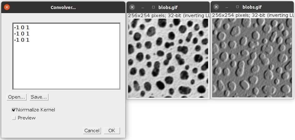
|
||||||
|
Here, I am going to show you how to create a fast convolution implementation that you can trivially augment to apply to any number of dimensions. Notice we import the offset operation from ImgMath, in addition to add and mul. With offset, we can summon values from another pixel by providing relative coordinates, e.g. [-1, 0] means "pick the value of the pixel to the left" (-1 in the X axis, 0 in the Y axis), for a 2D image. The operation right_edges adds up the multiplication of each nearby pixel by its corresponding weight according to the kernel. Some multiplications are not included as they multiply by 1, or not even added at all because they multiply by zero. So the add needs only 6 entries (3 of the 9 have zero weight). There's quite a bit of fiddling in setting up the operations. We can do much better.
|
from net.imglib2.algorithm.math.ImgMath import computeIntoFloats, add, offset, mul
from net.imglib2.img.display.imagej import ImageJFunctions as IL
from net.imglib2.view import Views
from ij import IJ

img = IL.wrap(IJ.getImage()) # E.g. blobs sample image
imgE = Views.extendBorder(img)

# Convolve with 3x3 kernel:
# -1 0 1
# -1 0 1
# -1 0 1
right_edges = add(mul(-1, offset(imgE, [-1, -1])),
                  mul(-1, offset(imgE, [-1,  0])),
                  mul(-1, offset(imgE, [-1,  1])),
                  offset(imgE, [1, -1]),
                  offset(imgE, [1, 0]),
                  offset(imgE, [1, 1]))

target = computeIntoFloats(right_edges)
IL.wrap(target, "right edges").show()
|
||||||
|
Now, let's create all four types of edges, using these kernels:
-1 0 1   -1 -1 -1   1 0 -1   1  1  1
-1 0 1    0  0  0   1 0 -1   0  0  0
-1 0 1    1  1  1   1 0 -1  -1 -1 -1
We define the function as2DKernel which takes an extended image as argument (via Views.extendedBorder so as to be able to cope with pixels near the border of the image without additional manual fiddling) and an array of odd length and of a length that is the square of the side of the 2D weight kernel to use. Returns an add of all weight mul of the corresponding pixel values read with offset (an offset op is merely shorthand for Views.translate). Note that later, under the hood, all multiplications by zero are pruned away, and those multiplied by one are merely replaced with the value that the 1 is multiplying. In other words, instead of manually having to specify (as we did above for right_edges) which pixels to skip (zero weight) or to not bother multiplying by the kernel weight (weight of 1), we can delegate that to the ImgMath machinery, resulting in simpler code that is easy to read, and general too: any 2D square kernels can be created with this function. Then we combine the ops for all four types of edges using either minimum or maximum, giving us black edges or white edges, respectively. Notice that none of the code here is specific of 2D dimensions, except for the as2DKernel function--which we could easily change to work in e.g. 3D. The rest of the code is dimension-independent. Note also that we can't use computeIntoFloats because there isn't an image limited to an interval within the operations: there is instead an extended image (a RandomAccessible in ImgLib2 parlance), and therefore ImgMath can't automatically determine the dimensions of the output image. So we provide one instead using compute...into in the combine function. Finally we run a rough segmentation by using old-school methods from ImageJ's menus: "convert to Mask" (a threshold) and "Fill Holes" (a binary operation). The result is not perfect, and some amount of fiddling could make it be for this sample, but it's not trivial and there will almost always be edge cases (blobs that don't get segmented or not properly). Instead, you should apply machine learning approaches to segmentation such as Trainable Segmentation. Or see below! |
from net.imglib2.algorithm.math.ImgMath import compute, add, offset, mul, minimum, maximum
from net.imglib2.img.display.imagej import ImageJFunctions as IL
from net.imglib2.type.numeric.real import FloatType
from net.imglib2.view import Views
from ij import IJ

img = IL.wrap(IJ.getImage()) # E.g. blobs sample image
imgE = Views.extendBorder(img)

def as2DKernel(imgE, weights):
  """ imgE: a RandomAccessible, such as an extended view of a RandomAccessibleInterval.
      weights: an odd-length list defining a square convolution kernel
               centered on the pixel, with columns moving slower than rows.
      Returns an ImgMath op.
  """
  # Check preconditions: validate kernel
  if 1 != len(weights) % 2:
    raise Error("list of kernel weights must have an odd length.")
  side = int(pow(len(weights), 0.5)) # sqrt
  if pow(side, 2) != len(weights):
    raise Error("kernel must be a square.")
  half = (side - 1) / 2
  # Generate ImgMath ops
  # Note that multiplications by weights of value 1 or 0 will be erased automatically
  # so that the hierarchy of operations will be the same as in the manual approach above.
  return add([mul(weight, offset(imgE, [index % side - half, index / side - half]))
              for index, weight in enumerate(weights)])


# All 4 edge detectors (left, right, top, bottom)
opTop = as2DKernel(imgE, [-1]*3 + [0]*3 + [1]*3)
opBottom = as2DKernel(imgE, [1]*3 + [0]*3 + [-1]*3)
opLeft = as2DKernel(imgE, [-1, 0, 1] * 3)
opRight = as2DKernel(imgE, [1, 0, -1] * 3)

def combine(op, title, *ops):
  edges_img = img.factory().imgFactory(FloatType()).create(img)
  compute(op(*ops)).into(edges_img)
  imp = IL.wrap(edges_img, title)
  imp.getProcessor().resetMinAndMax()
  imp.show()
  return imp

imp_max = combine(maximum, "max edges", opTop, opBottom, opLeft, opRight)
imp_min = combine(minimum, "min edges", opTop, opBottom, opLeft, opRight)

# Create a mask for blobs that don't contact the edges of the image
IJ.run(imp_mask, "Convert to Mask", "") # result has inverted LUT
IJ.run(imp_mask, "Fill Holes", "")
IJ.run(imp_mask, "Invert LUT", "") # revert to non-inverted LUT
imp_mask.show()
|
||||||
|
|
|
||||||
|
Block-reading integral images from ImgMath An integral image, also known as summed-area table, is "a data structure and algorithm for quickly and efficiently generating the sum of values in a rectangular subset of a grid". With integral images, Viola and Jones (2001) demonstrated "Robust Real-time Object Detection" by approximating otherwise costly image filters with similar, good-enough filters crafted from integral images. See also these excellent papers: "Integral channel features" by Dollar et al. (2009), "Integral Histogram: A Fast Way to Extract Histograms in Cartesian Spaces" by Porikli (2005), "Integral image-based representations" by Derpanis (2007), "Adaptive Thresholding Using the Integral Image" by Bradley and Roth (2007), "Prefix Sums and Their Applications" by Blelloch (1993), "Efficiently scaling edge detectors" by Kerr et al. 2010, "Non-orthogonal Binary Expansion of Gabor Filters with Applications in Object Tracking" by Tang and Tao, 2007, "Summed-area tables for texture mapping" by Crow (1984), and "A note on the computation of high-dimensional integral images" by Tapia 2011. The imglib2-algorithm repository offers the integral package with a general multi-dimensional IntegralImg class and two specializations for double and long primitive types. In the first example we illustrate the use of the integral image to blur an image by computing, for each pixel, the mean pixel intensity of a square centered on it. We construct an IntegralImg, extend its borders, and read blocks from it using ImgMath's block operation. You could think of this operation as a scale-area averaging (cheap) approach to approximating a Gaussian blur (expensive and accurate, using a radius). This plot shows the profile across the diagonal of the Gaussian blurred image (black) and the integral image-based block mean (red). They are different, but for some purposes it doesn't matter.
|
from net.imglib2.algorithm.math.ImgMath import compute, block, div
from net.imglib2.img.display.imagej import ImageJFunctions as IL
from net.imglib2.algorithm.integral import IntegralImg
from net.imglib2.type.numeric.integer import UnsignedLongType
from net.imglib2.type.numeric.real import FloatType
from net.imglib2.view import Views
from net.imglib2.algorithm.math.abstractions import Util
from ij import IJ

imp = IJ.getImage() # an 8-bit image, e.g. blobs sample image
img = IL.wrap(imp)

# A converter from 8-bit (unsigned byte) to 64-bit (unsigned long)
int_converter = Util.genericIntegerTypeConverter()
# Create the integral image of an 8-bit input, stored as 64-bit
alg = IntegralImg(img, UnsignedLongType(), int_converter)
alg.process()
integralImg = alg.getResult()

# Read out blocks of radius 5 (i.e. 10x10 for a 2d image)
radius = 5
nd = img.numDimensions()
op = div(block(Views.extendBorder(integralImg), [radius] * nd),
         pow(radius*2, nd))
blurred = img.factory().create(img) # an 8-bit image
# Compute in floats, store result into longs
# using a default generic RealType converter via t.setReal(t.getRealDouble())
# to map from input type to computing type (FloatType here), and
# from computing type to output type
compute(op).into(blurred, FloatType())

# Show the blurred image with the same LUT as the original
imp2 = IL.wrap(blurred, "integral image radius 5 blur")
imp2.getProcessor().setLut(imp.getProcessor().getLut())
imp2.show()


# Compare with Gaussian blur
from ij import ImagePlus
from ij.plugin.filter import GaussianBlur
from ij.gui import Line, ProfilePlot

# Gaussian of the original image
imp_gauss = ImagePlus(imp.getTitle() + " Gauss", imp.getProcessor().duplicate())
GaussianBlur().blurGaussian(imp_gauss.getProcessor(), radius)
imp_gauss.show()

# Plot values from a diagonal from bottom left to top right
line = Line(imp.getWidth() -1, 0, 0, imp.getHeight() -1)
imp_gauss.setRoi(line)
pp1 = ProfilePlot(imp_gauss)
plot = pp1.getPlot()
imp2.setRoi(line)
pp2 = ProfilePlot(imp2)
profile2 = pp2.getProfile() # double[]
plot.setColor("red")
plot.add("line", range(len(profile2)), profile2)
plot.show()
|
||||||
|
Note that, if your code merely requires integral images of 2D images, using ImageJ's data types like ImageProcessor, then Stephan Saalfeld wrote a high-performance library to do just that, providing integral image-based filters such as the mean, variance, standard deviation, remove outliers and normalize local contrast. You'll find these under Fiji's "Plugins - Integral image filters" menu. For completeness, here is an example using Saalfeld's integral image libray with its BlockStatistics class. There's also the Mean (so as to avoid computing the square integral image when not necessary, which BlockStatistics always does and which it needs for the variance and standard deviation), Scale and others, all based on integral images. |
from mpicbg.ij.integral import BlockStatistics
from ij import IJ, ImagePlus

imp = IJ.getImage() # e.g. the blobs sample image
radius = 5

# Works only with FloatProcessor
fp = imp.getProcessor().convertToFloat()
bs = BlockStatistics(fp)

# Write the mean for the given radius, in place:
bs.mean(radius) # or bs.mean(radius, radius) for different radii in X, Y

blurred = ImagePlus("blurred", fp)
blurred.show()

# see also methods:
# bs.std(radius)
# bs.variance(radius)
# bs.sampleVariance(radius)
|
||||||
|
Create an integral image with ImgMath While using IntegralImg should be your preferred approach, I show here how to create an n-dimensional plain integral image to illustrate the capabilities of ImgMath. For every pixel we add up it's value plus the value of the prior pixel, doing as many passes as dimensions the image has. I.e. first we add up in X, then we add up in Y, etc. This approach can work because ImgMath can write the result into an image that is also one of the input images, so the sums accummulate. Of course, this only works if the image is of a kind (like e.g. ArrayImg or PlanarImg) whose Cursor traverses its pixels in flat iteration order, namely, the lowest dimension (X) runs fastest when iterating over e.g. X, Y first the X increments until done with the first line, only then the Y increments and the X resets, and so on. (If your image is e.g. a CellImg whose iteration order isn't flat as required, you can acquire a flat-iterable view of it with the homonymous method Views.flatIterable.) Some of the filters we'll make require not a plain integral image, but the integral image of squares: first square the value of each pixel, then compute the integral image. Insert the pow op to wrap the reading of original img when copying into target, like this:
compute(pow(img, 2)).into(target)
|
from net.imglib2.algorithm.math.ImgMath import compute, block, div, offset, add
from net.imglib2.img.display.imagej import ImageJFunctions as IL
from net.imglib2.img.array import ArrayImgs
from net.imglib2.type.numeric.real import FloatType
from net.imglib2.view import Views
from net.imglib2.util import Intervals
from ij import IJ

imp = IJ.getImage() # an 8-bit image
img = IL.wrap(imp)

# Create the integral image of an 8-bit input, stored as 64-bit
target = ArrayImgs.unsignedLongs(Intervals.dimensionsAsLongArray(img))
# Copy input onto the target image
compute(img).into(target)
# Extend target with zeros, so that we can read at coordinate -1
imgE = Views.extendZero(target)
# Integrate every dimension, cummulatively by writing into
# a target image that is also the input image
for d in xrange(img.numDimensions()):
  coord = [0] * img.numDimensions() # array of zeros
  coord[d] = -1
  # Cummulative sum along the current dimension
  # Note that instead of the ImgMath offset op,
  # we could have used Views.translate(Views.extendZero(target), [1, 0]))
  # (Notice though the sign change in the translation)
  integral = add(target, offset(imgE, coord))
  compute(integral).into(target)

# The target is now the integral image
integralImg = target

# Read out blocks of radius 5 (i.e. 10x10 for a 2d image)
# in a way that is entirely n-dimensional (applies to 1d, 2d, 3d, 4d ...)
radius = 5
nd = img.numDimensions()
op = div(block(Views.extendBorder(integralImg), [radius] * nd),
         pow(radius*2, nd)) # divide by total number of pixels in the block

blurred = ArrayImgs.floats(Intervals.dimensionsAsLongArray(img))
compute(op).into(blurred, FloatType())

# Show the blurred image with the same LUT as the original
imp2 = IL.wrap(blurred, "integral image radius 5 blur")
imp2.getProcessor().setLut(imp.getProcessor().getLut())
imp2.show()
|
||||||
|
Intermezzo: machine learning with the WEKA library The WEKA library is an open source package for data mining with machine learning. It offers multilayer perceptrons (MultilayerPeceptron classifier; one of the oldest kind of neural network architectures), suport vector machines (SMO, by Platt 1998 and Keerthi et al. 2001), and Random Forests (RandomForest and FastRandomForest, after Breiman 2001), among many other classifiers (see classes implementing the Classifier interface). All classifiers operate similarly, but each has its own constructor and methods to adjust parameters. The basic premise of machine learning is that we have at hand a set of data points of known classification, to use as examples from which to infer, or learn, the underlying statistical distributions. Yes, machine learning is a subset of statistics by another name. In the WEKA library, we can describe each data point as a vector (a list) of scalars (numeric values), each described as an Attribute that can have a name (e.g. length, surface, weight, etc.; here merely "attr-1", "attr-2", etc.). The last attribute is the class, expressed as an index (in the case of each data point being described as a vector of scalars, as is the case here). When creating the attribute for the class, we give it the list of class names, ordered in a way that, later, the position of each class name in this list corresponds to the class index that we assign to each example data point. With the attributes, we construct an Instances object (here, training_data), which is a data structure containing both the attributes and the example data points. We add each data point as an Instance (an interface)--here, as a DenseInstance that takes the weight (ranging from 0 to 1, expressing how certain we are that this data point's class instance index is correct) and the vector of scalar values, one per attribute, with the class index as the last value of the vector. For this introductory example I've generated two random data sets. The first one (class index 0) is a set of 3-attribute data points whose scalar values range from 0 to 1, whereas for the second one (class index 1) they range from 1 to 2. We'll ask of the classifier to learn to differentiate between these two data sets. The classifier is an SMO, which more than suffices for this kind of data. With the training_data we can now invoke classifier.buildClassifier, which invokes the training of the classifier. (After this, you could save the trained classifier object to disk with SerializationHelper, for later use, to be reloaded using the same utility class.) All that remains now is to test whether the example data sufficed the train the chosen classifier. We construct again an Instances object named info containing the attributes and knowledge of which index in the vector of scalars of an instance is the class index, and with size 1 (i.e. containing a single data point). Then we create a DenseInstance for each test data point to classify (the test set test_samples), having first invoked setDataset(info) on it to provide the context it needs (namely, the attributes and classes). Finally, classifier.classifyInstance returns the class index that the classifier best estimates corresponds to the given data point. |
# Basic example of machine learning with the WEKA library

from jarray import array
from java.util import ArrayList, Random
from weka.core import Attribute, Instances, DenseInstance
from weka.classifiers.functions import SMO

# List of attributes: each is a value in a vector for each sample
n_attributes = 3
attributes = ArrayList([Attribute("attr-%i" % (i+1)) for i in xrange(n_attributes)])
# Plus the class, here only two classes with indices 0 and 1
attributes.add(Attribute("class", ["first", "second"]))

# Training data: each sample is a vector of 4 values (3 attributes and the class index).
# Here, two different distributions (two classes) are generated, whose attributes
# take values within [0, 1) (for class index 0) and within [1, 2) (for class index 1)
random = Random()
samples = [random.doubles(n_attributes, k, k+1).toArray() + array([k], 'd')
           for i in xrange(50) # 50 samples per class
           for k in (0, 1)] # two class indices

# The datastructure containing the training data
training_data = Instances("training", attributes, len(samples))
training_data.setClassIndex(len(attributes) -1) # the last one is the class
# Populate the training data, with all samples having the same weight 1.0
for vector in samples:
  training_data.add(DenseInstance(1.0, vector))

# The classifier: an SMO (support vector machine)
classifier = SMO()
classifier.buildClassifier(training_data)

# Test data
test_samples = [[0.5, 0.2, 0.9],   # class index 0
                [0.7, 0.99, 0.98], # class index 0
                [1.0, 1.2, 1.3],   # class index 1
                [1.6, 1.3, 1.1]]   # class index 1
# Umbrella data structure with the list of attributes
info = Instances("test", attributes, 1) # size of 1
info.setClassIndex(len(attributes) -1)

# Classify every test data sample
for vector in test_samples:
  instance = DenseInstance(1.0, vector) # vector list as double[] automatically
  instance.setDataset(info)
  class_index = classifier.classifyInstance(instance)
  print "Classified", vector, "as class", class_index
|
||||||
|
Segmentation with ImgMath and the WEKA machine learning library Above we segmented the sample "blobs" image using plain ImgMath filters, essentially a convolution with a kernel. While the results aren't bad, there are edge cases, i.e. blobs that don't get segmented. Here, we are going to test out the unreasonable effectiveness of machine learning (paraphrasing Sejnowski). First, we need example data. While generally for bioimagery this would mean manually annotated data (think ROIs), we can get away with synthetic data: data that looks close enough to the data of interest, and that we can generate in such a way that we know exactly e.g. which pixels belong to the structures to segment (the blobs) or the background. Or more precisely, if we can estimate closely enough the underlying generative process, we can tap into it (see e.g. Content Aware Image Restoration or CARE). Here, the positive examples are taken from an OvalRoi oval_inside that is one pixel shorter in radius relative to the blob we painted on the synth image, to ensure we pick pixels that belong to the blob itself rather than its boundary, which will help separate closely positioned blobs. For the negative examples, we picked a bunch of coordinates along the edge of a rectangular ROI between the painted blob (which is in the middle) and the edge of the image. Note the function asIntCoords gets the sequence of coordinates on a ROI and reads them as they are or as sampled at one pixel intervals along the lines of the ROI. The latter is useful because e.g. a plain ROI, which is rectangular, would only have 4 points (the 4 corners) whereas we need at least as many as along the oval_inside. But we want to balance the number of positive and negative examples used for training, so we crop the list using the limit keyword argument for the background examples, given that the rectangular ROI, sampled at every pixel, has far more coordinates than the much smaller oval_inside. The examples generator merely creates a joint list of pairs of coordinates on a 2D image and their class index, the latter being either 0 (for the blob) or 1 (for the background). Then we define a filter bank, that is, a set of measurements for every pixel (each of these will correspond to an attribute). Here, we define the function filterBankBlockStatistics which returns only two filters: the mean and the variance for a block (an area) centered on each pixel. These filters are created with ImgMath and integral images for fast computation that is independent of the block size. While we could use far more than merely two filters, turns out, for the sample blobs image, these more than suffice. The next few functions are all related to the WEKA machine learning library, which is included in Fiji. Most of the function bodies is busywork to shape our example data into data structures that the WEKA classifiers expect (Instances with their collections of Attribute and DenseInstance). The function sampleTrainingData takes the examples (a sequence of coordinates, each with a class index) as input (in its samples argument) and structures it into an Instances object, that packs along the number and names of attributes (each filter, that is, each entry into the vector of values for each pixel, here a vector of two values only plus the class index for that pixel), and the list of class_names. For simplicity (and speed, from jython), note I use Views.collapse over the Views.stack of all images, one per ImgMath filter or op. The collapse returns an imglib2 image of Composite: each pixel is a vector of scalar values. Note that, for performance, it would be best to use a java function to retrieve the array (the vector) of values for each example pixel, but given that we have very few examples, it doesn't matter. And further note a crucial performance feature: instead of materializing each filter (each op) into an image, instead we invoke op.view(FloatType()) for each, returning opViews: a list of RandomAccessibleInterval, one for each op, from which via a RandomAccess computed values can be retrieved at arbitrary coordinates. That is, we avoid computing each filter for every pixel of the img, and instead, we do so only for the pixel coordinates specified in the samples. This is possible, and even trivial, thanks to imglib2's abstractions, via ImgMath. (The cost we pay, for these kind of filters, is the creation of the integral images, which is an O(n) operation involving two integer sums per pixel: relatively cheap.) The functions trainClassifier and createSMOClassifier are convenient for creating a support vector machine (SVM) using the WEKA's SMO class and training with examples; the first of these two can be reused for any of the other classifiers offered by the WEKA library (of which there are many, including random forest, neural networks, and more). Note the optional argument filepath which, when not None, is used to serialize the trained classifier to disk for reusing it later (so that we don't have to relearn it every time we have to apply it to a new image of similar characteristics). Then we define the classify function, which takes an image and a WEKA classifier (or a string describing the filepath from which to load it), the filter bank ops, and the argument distrib_class_index to choose whether to get a result image where each pixel is the classified class index for that pixel, or the floating-point value within a distribution for a specific class index (useful for e.g. later applying your own thresholding methods such as graph cut from Lou et al. 2012). Finally, we use these generic functions: we generate filter banks (via ImgMath) for the training and test images, create and train the SMO classifier, print its internal details, and classify the blobs image. The result, considering how little training we used, how few filters, and that it was synthetic to begin with, is spectacularly good. That said, this particular "blobs.gif" sample image could have similarly have been segmented with a plain threshold, i.e. was not a challenging example. Yet, compared to edge detection with convolution and then attempting to combine the detections (see above), this approach has room to grow towards accommodating far more diverse and therefore more challenging data. At the end, I also show both images as a stack so that it's easier to visually evaluate the quality of the segmentation. Note we multiply the classification image resultSMO by 255, so that the segmentation (which has only values of 0 and 1, for background and blob respectively) is visible with the same min, max settings as the blobs image.
|
from ij import IJ, ImagePlus
from ij.process import FloatProcessor
from ij.gui import OvalRoi, Roi
from net.imglib2.img.display.imagej import ImageJFunctions as IL
from itertools import izip
from net.imglib2.algorithm.math.ImgMath import compute, block, IF, THEN, ELSE, LT, \
                                               sub, div, let, power, mul
from net.imglib2.algorithm.integral import IntegralImg
from net.imglib2.type.numeric.integer import UnsignedLongType, UnsignedByteType
from net.imglib2.view import Views
from net.imglib2.algorithm.math.abstractions import Util
from net.imglib2.img.array import ArrayImgs
from jarray import array
from java.util import ArrayList
from weka.core import SerializationHelper, DenseInstance, Instances, Attribute
from weka.classifiers.functions import SMO


# Synthetic training data: a bright blob on a black background
width, height = 64, 64
fp = FloatProcessor(width, height)
synth = ImagePlus("synth blob", fp)

fp.setColor(0)
fp.fill()
fp.setColor(255)
oval = OvalRoi(width/4, height/4, width/2, height/2)
fp.fill(oval)
fp.noise(25)

synth.show()

def asIntCoords(roi, asFloat=True, limit=-1):
  """ asFloat: enables sampling the ROI at e.g. 1.0 pixels intervals.
      limit: crop the number of points. """
  pol = roi.getInterpolatedPolygon(1.0, False) if asFloat else roi.getPolygon()
  coords = [map(int, points) for points in [pol.xpoints, pol.ypoints]]
  return coords[0][:limit], coords[1][:limit]

# Positive examples: an oval one pixel smaller in radius to sample
# from the inside boundary, to ensure nearby touching blobs are segmented separately
bounds = oval.getBounds()
oval_inside = OvalRoi(bounds.x + 1, bounds.y + 1, bounds.width - 1, bounds.height - 1)
blob_boundary = asIntCoords(oval_inside, asFloat=False)
print len(blob_boundary[0])

# Negative examples: as many as positive ones,
# well oustide the oval but also far from the border
margin = min(width/8, height/8)
background_roi = Roi(margin, margin, width - margin, height - margin)
background = asIntCoords(background_roi, asFloat=True, limit=len(blob_boundary[0]))

class_names = ["boundary", "background"]

def examples():
  """ A generator sequence of pairs of coordinates and their
      corresponding class index. """
  for class_index, (xs, ys) in enumerate([blob_boundary, background]):
    for x, y in izip(xs, ys):
      yield [x, y], class_index


def filterBankBlockStatistics(img, block_width=5, block_height=5,
                              sumType=UnsignedLongType(),
                              converter=Util.genericRealTypeConverter()):
  # corners of a block centered at the pixel
  block_width = int(block_width)
  block_height = int(block_height)
  w0 = -block_width/2  # e.g. -2 when block_width == 4 and also when block_width == 5
  h0 = -block_height/2
  decX = 1 if 0 == block_width  % 2 else 0
  decY = 1 if 0 == block_height % 2 else 0
  w1 = block_width/2  - decX # e.g. 2 when block_width == 5 but 1 when block_width == 4
  h1 = block_height/2 - decY

  corners = [[w0, h0], [w1, h0],
             [w0, h1], [w1, h1]]

  # Create the integral image, stored as 64-bit
  alg = IntegralImg(img, sumType, converter)
  alg.process()
  integralImgE = Views.extendBorder(alg.getResult())

  # Create the integral image of squares, stored as 64-bit
  sqimg = compute(power(img, 2)).view(sumType)
  algSq = IntegralImg(sqimg, sumType, converter)
  algSq.process()
  integralImgSqE = Views.extendBorder(algSq.getResult())

  # block mean: creates holes in blurred membranes
  opMean = div(block(integralImgSqE, corners), block_width * block_height)

  # block variance: sum of squares minus square of sum
  opVariance = sub(block(integralImgSqE, corners), power(block(integralImgE, corners), 2))
  opVarianceNonZero = let("var", opVariance,
                          IF(LT("var", 0),
                             THEN(0),
                             ELSE("var")))

  return [opMean, opVarianceNonZero]


def sampleTrainingData(img, samples, class_names, ops, n_samples=0):
  """ img: a 2D RandomAccessibleInterval.
      samples: a sequence of long[] (or int numeric sequence or Localizable)
               and class_index pairs; can be a generator.
      class_names: a list of class names, as many as different class_index.
      ops: the sequence of ImgMath ops to apply to the img.
      n_samples: optional, the number of samples (in case samples is e.g. a generator).

      Return an instance of WEKA Instances, each consisting in a vector
      of values (one per op) for every sample over the img.
  """
  if 0 == n_samples:
    n_samples = len(samples)

  # Define a WEKA Attribute for each feature (one for op in the filter bank, plus the class)
  attribute_names = ["attr-%i" % (i+1) for i in xrange(len(ops))]
  attributes = ArrayList()
  for name in attribute_names:
    attributes.add(Attribute(name))
  # Add an attribute at the end for the classification classes
  attributes.add(Attribute("class", class_names))

  # Create the training data structure
  training_data = Instances("training", attributes, n_samples)
  training_data.setClassIndex(len(attributes) -1)

  # A RandomAccess on a Composite view of FloatType views of every ImgMath op
  # (i.e. no need to compute each op for all pixels of the img!
  #  Will instead compute only for the sampled pixels.)
  opViews = [op.view(FloatType()) for op in ops]
  ra = Views.collapse(Views.stack(opViews)).randomAccess()

  for position, class_index in samples:
    ra.setPosition(position)
    tc = ra.get()
    vector = array((tc.get(i).getRealDouble() for i in xrange(len(opViews))), 'd')
    vector += array([class_index], 'd') # inefficient, but easy
    training_data.add(DenseInstance(1.0, vector))

  return training_data


def trainClassifier(classifier, img, samples, class_names, ops, n_samples=0, filepath=None):
  classifier.buildClassifier(sampleTrainingData(img, samples, class_names, ops, n_samples=n_samples))

  # Save the trained classifier for later
  if filepath:
    SerializationHelper.write(filepath, classifier)

  return classifier


def createSMOClassifier(img, samples, class_names, ops, n_samples=0, filepath=None):
  """ Create a classifier: support vector machine (SVM, an SMO in WEKA)

      img: a 2D RandomAccessibleInterval.
      samples: a sequence of long[] (or int numeric sequence or Localizable)
               and class_index pairs; can be a generator.
      class_names: a list of class names, as many as different class_index.
      ops: a list of ImgMath operations, each one is a filter on the img.
      n_samples: optional, the number of samples (in case samples is e.g. a generator).
      save_to_file: optional, a filename for saving the learnt classifier.
  """
  return trainClassifier(SMO(), img, samples, class_names, ops,
                         n_samples=n_samples, filepath=None)


def classify(img, classifier, class_names, ops, distrib_class_index=-1):
  """ img: a 2D RandomAccessibleInterval.
      classifier: a WEKA Classifier instance, like SMO or FastRandomForest, etc. Any.
                  If it's a string, interprets it as a file path and attempts to deserialize
                  a previously saved trained classifier.
      class_names: the list of names of each class to learn.
      ops: the filter bank of ImgMath ops for the img.
      distrib_class_index: defaults to -1, meaning return the class index for each pixel.
                           When larger than -1, it's interpreted as a class index, and
                           returns instead the floating-point value of each pixel in
                           the distribution of that particular class index. """
  if type(classifier) == str:
    classifier = SerializationHelper.read(classifier)

  attributes = ArrayList()
  for i in xrange(len(ops)):
    attributes.add(Attribute("attr-%i" % i))
  attributes.add(Attribute("class", class_names))

  # Umbrella datastructure "Instances" containing the attributes of each "Instance" to classify
  # where an "Instance" will be each pixel in the image.
  info = Instances("structure", attributes, 1)
  info.setClassIndex(len(attributes) -1)

  # Compute all ops and stack them into an imglib2 image of CompositeType
  # where every "pixel" is the vector of all op values for that pixel
  opImgs = [compute(op).into(ArrayImgs.floats([img.dimension(0), img.dimension(1)]))
            for op in ops]
  cs_opImgs = Views.collapse(Views.stack(opImgs))

  classification = ArrayImgs.floats([img.dimension(0), img.dimension(1)])
  cr = classification.cursor()
  cop = Views.iterable(cs_opImgs).cursor()

  # For every pixel in the image
  while cr.hasNext():
    tc = cop.next()
    vector = array((tc.get(i).getRealDouble() for i in xrange(len(opImgs))), 'd')
    vector += array([0], 'd') # for the class, which is at the end
    di = DenseInstance(1.0, vector)
    di.setDataset(info) # the list of attributes
    if distrib_class_index > -1:
      cr.next().setReal(classifier.distributionForInstance(di)[distrib_class_index])
    else:
      cr.next().setReal(classifier.classifyInstance(di))

  return classification # an image, where each pixel is the corresponding class index


# The training image: our synthetic blob
img_training = IL.wrap(synth)

# The test image: the sample image "blobs.gif"
blobs_imp = IJ.openImage("http://imagej.nih.gov/ij/images/blobs.gif")
img_test = IL.wrap(blobs_imp)

# The same filter bank for each
ops_training = filterBankBlockStatistics(img_training)
ops_test = filterBankBlockStatistics(img_test)

# The WEKA support vector machine (SVM) named SMO
classifierSMO = createSMOClassifier(img_training, examples(), class_names, ops_training,
                                    n_samples=len(blob_boundary[0]),
                                    filepath="/tmp/svm-blobs-segmentation")
print classifierSMO.toString()

# Classify pixels as blob boundary or not
resultSMO = classify(img_test, classifierSMO, class_names, ops_test)
IL.wrap(resultSMO, "segmentation via WEKA SVM SMO").show()

# Better display as a stack
stack = Views.stack(img_test,
                    compute(mul(resultSMO, 255)).view(UnsignedByteType()))
IL.wrap(stack, "stack").show()
|
||||||
|
Segmenting an electron micrograph of nervous tissue using ImgMath and WEKA Let's try now a far more challenging problem: segmenting neurons in an electron microscopy image of a single 40-nm serial section of neural tissue. As in the blobs segmentation example, we are going to need examples, in this case of what is a membrane and what isn't, in order to train a classifier. For the purpose, as before, I am going to make up some data: a synthetic image that imitates (eyeballing it!) how cytoplasmic membranes look like in transmission electron micrographs. The motivation for the specifics of the synthetic data for training comes from a couple of rough measurements of membrane thickness (in pixels), both when sectioned orthogonally (sharp and dark) or more oblique (difuse and far less dark). Multiple contacting ovals serve the purpose of representing adjacent cytoplasmic membranes. Perhaps unnecessarily, but to potentially add some realism, I sprinke faint vesicles, then Gaussian-blur the image, and then inject shot noise. Most of these are accomplished using ImageJ's ImageProcessor methods for drawing ROIs of a specified line width and color, and noise. The GaussianBlur is a built-in ImageJ plugin.
From the ROIs used to draw the synthetic membranes we can now sample data for membrane and membrane_oblique. For the background (nonmem) we sample points from a rectangular ROI defined to lay between the image border and the oval ROIs, not touching either. For balancing, I choose to sample the same amount of background locations as the amount of membrane and membrane_oblique combined. With the synthetic training data ready, we now proceed to train a WEKA MultilayerPerceptron. I've chosen this merely to illustrate its use; the SMO or FastRandomForest would do as well or better as a first attempt. Note that we reuse functions defined in the ImgMath blobs segmentation example above, namely the trainClassifier and classify. For the script to work, you'll have to copy-paste them and their imports (bad practice!) or instead, save those functions into a library file and import it as explained above. As for the inputs to the MultilayerPerceptron, I've chosen a block of the raw pixels centered on each pixel, of width 5 (so 25 pixels). This is managed here with the function readPatch which returns a list of ImgMath ops, namely a list of appropriately set ImgMath.offset, each reading one pixel of the block. Each pixel in the block becomes an Attribute for training. In other words: instead of applying filters as in the blobs example above, we feed the raw data as input to the perceptron. There are 3 classes: "membrane", "membrane_oblique" and "nonmem", with their corresponding class index (0, 1 and 2). The samples generator provides all pairs of coordinates and class index as required by trainClassifier inside the createPerceptronClassifier function. Most of the above may seem "just so", and it is: I put little effort if any into parameter exploration. I merely came up with training data that seemed reasonable, plus a way of feeding the data that was the simplest possible (a block of plain raw data around each pixel), and then chose a multi-layer architecture pretty much at random, with a first hidden layer (the one that first integrates the input) 3 times larger than the number of inputs (inspired by the Drosophila Kenyon cells, which are a large multiple of the number of projection neurons that feed into them; Eichler et al. 2017), a middle layer merely 1.5 that of the number of inputs, and then a third layer (just because) that is again 3 times the number of inputs. The output is merely 3 nodes (the 3 classes), so there's enormous convergence at the end. Despite this completely arbitrary choice of network, made up synthetic training data and no filters, the results are surprisingly good: membranes are indeed segmented (in black) and most cytoplasm structure is suppressed; an outcome that is pretty much what I wanted. There are here and there some nicks on the membranes, which result in merge errors: adjacent neurons are fused. Mitochondria weren't dealt with either. And, if you were to set a single hiden layer with 5 nodes (e.g. hidden_layers = "5"), you'd be surprised to get a nearly identical result, perhaps with more nicks in membranes but not many more. Trains and applies an order of magnitude faster too. Crucially, and unlike for the trivial blobs example earlier, no conventional thresholding algorithm would give such a result.
To improve this preliminary result you'll need to do parameter exploration regarding the structure of the multi-layer perceptron, and of course maybe feed in proper training data to begin with (so that it's as rich as possible, capturing all variations of membranes), as well as more carefully selected inputs (i.e. perhaps filters, like in the blobs example above). For reference, the winning entry of the ISBI 2012 challenge (Ciresan et al. 2012) used, for this very same image, a very deep and structured neural network consisting of a sequence of alternating convolutional and max-pooling layers, into which many transformed views (think barrel deformations and foveations) of rather large block patches centered at each pixel were fed, and used manual segmentations for the coordinates of training samples; the training time was measured in hundreds of minutes in a GPU (whereas here we are using a single-threaded implementation taking a few seconds). Note you'll need to have the "180-220-sub512x512-30.tif" image open, so that the script can grab it by its name with WindowManager.getImage. This image is available as part of a 30-image stack, as it was used for the ISBI 2012 image segmentation challenge. |
# Generate synthetic data emulating an electron microscopy image
# of a serial section of dense neural tissue
from ij import IJ, ImagePlus
from ij.process import FloatProcessor
from ij.gui import OvalRoi, Roi
from ij.plugin.filter import GaussianBlur
from java.util import Random

w, h = 128, 128
fp = FloatProcessor(w, h)
imp_synth = ImagePlus("synth training", fp)

fp.setColor(150) # background
fp.fill()

# neurites
rois = [OvalRoi(w/2 - w/4, h/2 - h/4, w/4, h/2), # stretched vertically
        OvalRoi(w/2, h/2 - h/8, w/4, h/4),
        OvalRoi(w/2 - w/18, h/2 + h/10, w/6, h/4),
        OvalRoi(w/2 - w/18, h/8 + h/16, w/3, h/5)]

fp.setColor(50) # membrane
fp.setLineWidth(3)

for roi in rois:
  fp.draw(roi)

fp.setColor(90) # oblique membrane
fp.setLineWidth(5)
roi_oblique = OvalRoi(w/2 + w/8, h/2 + h/8, w/4, h/4)
fp.draw(roi_oblique)

# Add noise
# 1. Vesicles
fp.setLineWidth(1)
random = Random(67779)
for i in xrange(150):
  x = random.nextFloat() * (w-1)
  y = random.nextFloat() * (h-1)
  fp.draw(OvalRoi(x, y, 4, 4))

fp.setRoi(None)

# 2. blur
sigma = 1.0
GaussianBlur().blurFloat(fp, sigma, sigma, 0.02)
# 3. shot noise
fp.noise(25.0)

fp.setMinAndMax(0, 255)
imp_synth.show()

# 3 classes, to which we'll assign later indices 0, 1, 2:
# Class 0. Membrane, from the ovals: 312 points
membrane = reduce(lambda cs, pol: [cs[0] + list(pol.xpoints), cs[1] + list(pol.ypoints)],
                  [roi.getPolygon() for roi in rois], [[], []])

# Class 1. Membrane oblique, fuzzy: another 76 points
membrane_oblique = reduce(lambda cs, pol: [cs[0] + list(pol.xpoints), cs[1] + list(pol.ypoints)],
                  [roi.getPolygon() for roi in [roi_oblique]], [[], []])

len_membrane = len(membrane[0]) + len(membrane_oblique[0])

# Class 2. Background samples: as many as membrane samples
rectangle = Roi(10, 10, w - 20, h - 20)
pol = rectangle.getInterpolatedPolygon(1.0, False) # 433 points
nonmem = (list(int(x) for x in pol.xpoints)[:len_membrane],
          list(int(y) for y in pol.ypoints)[:len_membrane])


# Machine learning: learn to classify neuron membranes from the synthetic samples
from weka.classifiers.functions import MultilayerPerceptron
from net.imglib2.algorithm.math.ImgMath import offset
from net.imglib2.view import Views
from net.imglib2.img.display.imagej import ImageJFunctions as IL
import os, tempfile
from itertools import izip
from ij import WindowManager

#####
# NOTE: these functions were defined above but are used here:
#    trainClassifier
#    sampleTrainingData
#    classify
# Please put them in a file along with their imports,
# then import only these two functions like e.g.:
#
# from mylib import classify, trainClassifier
#
# In my setup, I'd do this:
# import sys
# sys.path.append("/home/albert/lab/scripts/python/imagej/IsoView-GCaMP/")
# from lib.segmentation_em import classify, trainClassifier
#
# See: https://github.com/acardona/scripts/
#####


# A generator of training samples: coords over the ROIs and their class index
def samples():
  for class_index, (xs, ys) in enumerate([membrane, membrane_oblique, nonmem]):
    for x, y in izip(xs, ys):
      yield [x, y], class_index

class_names = ["membranes", "mem_oblique", "nonmem"]


def createPerceptronClassifier(img, samples, class_names, ops,
                               n_samples=0, filepath=None, params={}):
  mp = MultilayerPerceptron()
  if "learning_rate" in params:
    # In (0, 1]
    mp.setLearningRate(params.get("learning_rate", mp.getLearningRate()))
  # Number of nodes per layer: a set of comma-separated values (numbers), or:
  # 'a' = (number of attributes + number of classes) / 2
  # 'i' = number of attributes,
  # 'o' = number of classes
  # 't' = number of attributes + number of classes.
  # See MultilayerPerceptron.setHiddenLayers
  # https://weka.sourceforge.io/doc.dev/weka/classifiers/functions/MultilayerPerceptron.html#setHiddenLayers-java.lang.String-
  # Default hiddern layers: 3x,1.5x,3x the number of ops
  hidden_layers = "%i,%i,%i" % (len(ops) * 3, int(len(ops) * 1.5 + 0.5), len(ops) * 3)
  mp.setHiddenLayers(params.get("hidden_layers", hidden_layers))
  return trainClassifier(mp, img, samples, class_names, ops=ops,
                         n_samples=n_samples, filepath=filepath)


def readPatch(img, width=5):
  """ Returns as many ops as pixels within a square block of pixels (a patch)
      centered each pixel, each reading the plain pixel value. """
  half = width / 2 # e.g. for 5, it's 2
  imgE = Views.extendBorder(img)
  ops = [offset(imgE, [x, y]) for x in xrange(-half, half + 1)
                              for y in xrange(-half, half + 1)]
  return ops


# Train a multi-layer perceptron with the synthetic data
img_synth = IL.wrap(imp_synth)
ops = readPatch(img_synth, width=5)
hidden_layers = "%i,%i,%i" % (len(ops) * 3, int(len(ops) * 1.5 + 0.5), len(ops) * 3)
params = {"learning_rate": 0.5,
          "hidden_layers": hidden_layers
         }
filepath = os.path.join(tempfile.gettempdir(), "mp-mem-nonmem")
classifierMP = createPerceptronClassifier(img_synth, samples(), class_names, ops,
                                          n_samples=len(membrane[0]),
                                          filepath=filepath,
                                          params=params)
print classifierMP.toString()

# Apply the trained perceptron to the EM image
# ASSUMES the image 180-220-sub512x512-30.tif is open
imgEM = IL.wrap(WindowManager.getImage("180-220-sub512x512-30.tif"))
ops = readPatch(imgEM, width=5)

resultMP = classify(imgEM, classifierMP, class_names, ops=ops,
                    distribution_class_index=-1)
IL.wrap(resultMP, "Multi-layer perceptron segmentation").show()
|
||||||
|
Let's attempt to improve the above result by merely adjusting the input. My aim is to mitigate nicks in segmented membranes, which is the source of merge errors: two neuronal arbors being segmented erroneously as if they were one instead. My intuition is to try to better represent how membranes look like in the input to the classifier. To this end, we'll input filterBankBlockStatistics of rectangular blocks. And because such blocks can only be horizontal or vertical, we'll rotate the images and acquire blocks on those rotations, which is equivalent to feeding in rotated blocks. With this approach, naively, I expect to better capture the statistics of membranes, so that I don't have to rely on a most likely underpowered artificial neural network (the just-so, trivially small multi-layer perceptron) to extract such statistics, and instead have it focus on distinguishing membrane from non-membrane on the basis of such block statistics. The filterBankRotations takes as arguments an image, a function that generates ImgMath ops when invoked with the image as argument, and optional list of angles (in degrees) for the rotations, and the optional outputType for computing the rotations. Then, for each angle, a rotated view of each op (imgRot) is materalized into an ArrayImg (imgOpRot), and an unrotated (by minus the angle, back to the original pose) view (imgOpUnrot) is stored in the list of rotations (ops_rotations), which is returned when all angles and ops are processed. The list ops_rotations is as long as the number of ops times the number of angles. Given that we made the number of hidden_layers dependent on the number of ops, the structure of the multi-layer perceptron will be different. Before, there were 25 ops (5x5 pixel block), whereas now there are 7 angles times 2 ops (from filterBankBlockStatistics), so only 14 ops: the network is actually smaller, and will train faster than before. It worked; at least, the result is better. Below, top-right is the earlier result from a 5x5 block of raw pixels. Bottom left is the result of the rotated long blocks. Bottom right is both combined with a minimum function. Black is class 0 (membrane), grey is class 1 (membrane oblique), and white is class 2 (non-membrane).
While the results of the block statistics aproach are better (less membrane nicks), they aren't perfect: but the training data wasn't either. It's clear that more samples for oblique, faint membranes are necessary. If anything, it's remarkable how well the segmentation went. And combining the result of multiple classifiers is one strategy to patch up shortcommings of each one. |
# CONTINUES from above

from net.imglib2.realtransform import AffineTransform2D
from net.imglib2.realtransform import RealViews as RV
from net.imglib2.util import Intervals
from net.imglib2.interpolation.randomaccess import NLinearInterpolatorFactory
from net.imglib2.type.numeric.real import FloatType
from net.imglib2.algorithm.math.ImgMath import compute, minimum
from itertools import product, repeat
from jarray import array, zeros
from java.util import ArrayList
from math import radians, floor, ceil

####
# Note, as before, you'll need to import also this function
# that was defined above, e.g. if you save it in mylib.py then
from mylib import filterBankBlockStatistics
####


def rotatedView(img, angle, enlarge=True, extend=Views.extendBorder):
  """ Return a rotated view of the image, around the Z axis,
      with an expanded (or reduced) interval view so that all pixels are exactly included.

      img: a RandomAccessibleInterval
      angle: in degrees
  """
  cx = img.dimension(0) / 2.0
  cy = img.dimension(1) / 2.0
  toCenter = AffineTransform2D()
  toCenter.translate(-cx, -cy)
  rotation = AffineTransform2D()
  # Step 1: place origin of rotation at the center of the image
  rotation.preConcatenate(toCenter)
  # Step 2: rotate around the Z axis
  rotation.rotate(radians(angle))
  # Step 3: undo translation to the center
  rotation.preConcatenate(toCenter.inverse())
  rotated = RV.transform(Views.interpolate(extend(img),
                         NLinearInterpolatorFactory()), rotation)
  if enlarge:
    # Bounds:
    bounds = repeat((sys.maxint, 0)) # initial upper- and lower-bound values
                                     # for min, max to compare against
    transformed = zeros(2, 'f')
    for corner in product(*zip(repeat(0), Intervals.maxAsLongArray(img))):
      rotation.apply(corner, transformed)
      bounds = [(min(vmin, int(floor(v))), max(vmax, int(ceil(v))))
                for (vmin, vmax), v in zip(bounds, transformed)]
    minC, maxC = map(list, zip(*bounds)) # transpose list of 2 pairs
                                         # into 2 lists of 2 values
    imgRot = Views.zeroMin(Views.interval(rotated, minC, maxC))
  else:
    imgRot = Views.interval(rotated, img)
  return imgRot


def filterBankRotations(img,
                        filterBankFn, # function that takes an img as sole positional argument
                        angles=xrange(0, 46, 9), # sequence, in degrees
                        outputType=FloatType()):
  """ img: a RandomAccessibleInterval.
      filterBankFn: the function from which to obtain a sequence of ImgMath ops.
      angles: a sequence of angles in degrees.
      outputType: for materializing rotated operations and rotating them back.

      For every angle, will prepare a rotated view of the image,
      then create a list of ops on the basis of that rotated view,
      then materialize each op into an image so that an unrotated view
      can be returned back.

      returns a list of unrotated views, each containing the values of applying
      each op to the rotated view.
  """
  ops_rotations = []

  for angle in angles:
    imgRot = img if 0 == angle else rotatedView(img, angle)
    ops = filterBankFn(imgRot)

    # Materialize these two combination ops and rotate them back (rather, a rotated view)
    interval = Intervals.translate(img, [(imgRot.dimension(d) - img.dimension(d)) / 2
                                         for d in xrange(img.numDimensions())])
    for op in ops:
      imgOpRot = compute(op).intoArrayImg(outputType)
      if 0 == angle:
        ops_rotations.append(imgOpRot)
        continue
      # Rotate them back and crop view
      imgOpUnrot = rotatedView(imgOpRot, -angle, enlarge=False)
      imgOp = Views.zeroMin(Views.interval(imgOpUnrot, interval))
      ops_rotations.append(imgOp)

  return ops_rotations


def makeOps(img, angles):
  # Block statistics of rotations of an elongated block
  opsFn = lambda img: filterBankBlockStatistics(img, block_width=3,
                                                     block_height=7)
  ops = filterBankRotations(img, angles=angles, filterBankFn=opsFn)
  # Plain block statistics of a small square block
  ops += filterBankBlockStatistics(img, block_width=3, block_height=3)
  return ops

# List of angles for rotations
angles = [0, 15, 30, 45, 60, 75, 90]

# Train the multi-layer perceptron
ops = makeOps(img_synth, angles)
params = {"learning_rate": 0.5,
          "hidden_layers": "%i,%i,%i" % (len(ops) * 3, int(len(ops) * 1.5 + 0.5), len(ops) * 1)
         }
classifierMP = createPerceptronClassifier(img_synth, samples(), class_names, ops=ops,
                                          n_samples=len(membrane[0]),
                                          filepath="/tmp/mp-mem-nonmem-rotations-%s" % "-".join(map(str, angles)),
                                          params=params)
print classifierMP.toString()

# Apply the classifier to the electron microscopy image of nervous tissue
impEM = WindowManager.getImage("180-220-sub512x512-30.tif")
imgEM = IL.wrap(impEM)
ops = makeOps(imgEM, angles)
resultMProtations = classify(imgEM, classifierMP, class_names, ops=ops, distribution_class_index=-1)
IL.wrap(resultMProtations, "Multi-layer perceptron segmentation angles=%s" % str(angles)).show()


# combine them: the minimum of the two
combined = compute(minimum(resultMP, resultMProtations)).intoArrayImg()
IL.wrap(combined, "minimum of the two").show()
|
||||||
|
Create a virtual image pyramid from an integral image using ImgMath and imglib2 Image pyramids are a useful data structure that, downstream in the processing pipeline, lets us keep the dimensions of the features to extract constant (which simplifies computing), while reducing instead the dimensions of the images to analyze. The effect is the reverse, namely, the features extracted at higher pyramid levels (smaller images) are correspondingly larger because they include a larger area of the scene. Why generate image pyramids with ImgMath? The key feature lays in that all images here are actually views: no computations have happened yet. If downstream processing reads the pyramids only once, this will make no difference; if they were to read them more than once, you'll pay the cost of repeated computation (and a cheap one at that) but with the advantage of not having these pyramids stored in memory (a trade-off that you have to balance); if you were to require only a subset of the pyramid levels, or of the area of each image, and only once, they this approach both simplifies code and improves performance by avoiding unnecessary computations. The typical way of generating image pyramids is by blurring (e.g. with a Gaussian) and then subsampling (e.g. taking every other pixel). Here, we first compute an IntegralImg, and then we use Views.subsample to pick every second, every fourth, every eight, etc. pixel from a correspondingly larger ImgMath block. In other words, we view each level of the pyramid by generating it on the fly, computed from the additions and subtractions of the 4 corners of a square block read on the integral image. Because of how Then we show the images ordered in a grid, zooming in and enlarging the container window the right amount for each level of the pyramid, so that we can compare the degradation of image quality as we go up in levels of the pyramid. Note the magnification of each window; the original is the top left one. Sorting Fiji image windows into a grid is done by using methods from the ImageCanvas and ImageWindow, run within java's event dispatch thread via SwingUtilities.invokeLater. If you are interested in these test images, they are available; they were central to the ISBI 2012 image segmentation challenge.
|
from net.imglib2.algorithm.math.ImgMath import compute, block, div, offset, add
from net.imglib2.algorithm.math.abstractions import Util
from net.imglib2.algorithm.integral import IntegralImg
from net.imglib2.img.display.imagej import ImageJFunctions as IL
from net.imglib2.type.numeric.integer import UnsignedByteType, \
                          UnsignedShortType, UnsignedLongType
from net.imglib2.view import Views
from ij import IJ

imp = IJ.getImage() # e.g. EM of Drosophila neurons 180-220-sub512x512-30.tif
img = compute(IL.wrap(imp)).intoImg(UnsignedShortType()) # in 16-bit

# Create an integral image in longs
alg = IntegralImg(img, UnsignedLongType(), Util.genericIntegerTypeConverter())
alg.process()
integralImg = alg.getResult()

# Create an image pyramid as views, with ImgMath and imglib2,
# which amounts to scale area averaging sped up by the integral image
# and generated on demand whenever each pyramid level is read.
width = img.dimension(0)
min_width = 32
imgE = Views.extendBorder(integralImg)
blockSide = 1
# Corners for level 1: a box of 2x2
corners = [[0, 0], [1, 0], [0, 1], [1, 1]]
pyramid = [] # level 0 is the image itself, not added

while width > min_width:
  blockSide *= 2
  width /= 2
  # Scale the corner coordinates to make the block larger
  cs = [[c * blockSide for c in corner] for corner in corners]
  blockRead = div(block(imgE, cs), pow(blockSide, 2)) # the op
  # a RandomAccessibleInterval view of the op, computed with shorts but seen as bytes
  view = blockRead.view(UnsignedShortType(), UnsignedByteType())
  # Views.subsample by 2 will turn a 512-pixel width to a 257 width,
  # so crop to proper interval 256
  level = Views.interval(Views.subsample(view, blockSide),
                         [0] * img.numDimensions(), # min
                         [img.dimension(d) / blockSide -1
                          for d in xrange(img.numDimensions())]) # max
  pyramid.append(level)

# Show each pyramid level
#for i, level in enumerate(pyramid):
#  IL.wrap(level, str(i+1)).show()


# Instead, show and position the original window
# and each level of the pyramid in a 3x2 grid, zoomed in
from java.lang import Runnable
from javax.swing import SwingUtilities

offsetX, offsetY = 100, 100 # from top left of the screen, in pixels
gridWidth = 3
imp.getWindow().setLocation(offsetX, offsetY) # from top left

# Show each pyramid level
imps = [imp] + [IL.wrap(level, str(i+1)) for i, level in enumerate(pyramid)]

class Show(Runnable):
  def __init__(self, i, imp):
    self.i = i # index in the 3x2 grid, from 0 to 5
    self.imp = imp
  def run(self):
    self.imp.show()
    win = self.imp.getWindow()
    # zoom in so that the window has the same dimensions as the original image
    scale = int(pow(2, self.i))
    win.getCanvas().setMagnification(scale)
    win.getCanvas().setSize(self.imp.getWidth() * scale, self.imp.getHeight() * scale)
    win.pack()
    win.toFront()
    win.setLocation(offsetX + (self.i % gridWidth) * win.getWidth(),
                    offsetY + (self.i / gridWidth) * win.getHeight())

for i, imp in enumerate(imps):
  SwingUtilities.invokeLater(Show(i, imp))
|
||||||
|
Create an image pyramid with plain ImgLib2 For comparison with the above ImgMath integral image approach with area averaging, here is how to generate a sequence of pyramid levels using interpolated views (again, not the standard approach of Gaussian blur followed by subsampling). The approach relies on on-the-fly interpolation of each pixel in the downscaled images by using RealViews.transform with a Scale transformation of using non-linear interpolation via NLinearInterpolatorFactory. Note the scaled view is unbounded, i.e. it isn't an Interval (it's a transformation with interpolation of an extended view of the original image), and therefore we must bound (i.e. define an interval) the view of the scaled image (the level of the pyramid) with Views.interval, which takes as argument the scaled-down dimensions. As in the ImgMath case above, each "image" in the pyramid is merely a view (the level), but here, we materialize it into an actual image scaledImg, because otherwise e.g. the last and smallest level, to generate it, would have to generate all prior levels again. Before, each level was generated directly from the integral image with area averaging, whereas now the scaling is done via non-linear interpolation of the prior level. |
from net.imglib2.img.display.imagej import ImageJFunctions as IL
from net.imglib2.view import Views
from net.imglib2.realtransform import RealViews, ScaleAndTranslation
from net.imglib2.interpolation.randomaccess import NLinearInterpolatorFactory
from net.imglib2.util import ImgUtil
from net.imglib2 import FinalInterval
from ij import IJ

img = IL.wrap(IJ.getImage())

pyramid = [img] # level 0 is the image itself

# Create levels of a pyramid with interpolation
width = img.dimension(0)
min_width = 32

s = [0.5 for d in xrange(img.numDimensions())]
t = [-0.25 for d in xrange(img.numDimensions())]
while width > min_width:
  width /= 2
  imgE = Views.interpolate(Views.extendBorder(img), NLinearInterpolatorFactory())
  # A scaled-down view of the imgE
  level = Views.interval(RealViews.transform(imgE, ScaleAndTranslation(s, t)),
                         FinalInterval([int(img.dimension(d) * 0.5)
                                        for d in xrange(img.numDimensions())]))
  # Create a new image for this level
  scaledImg = img.factory().create(level) # empty, of dimensions as of level
  ImgUtil.copy(level, scaledImg) # copy the scaled down view (level) into scaledImg
  pyramid.append(scaledImg)
  # Prepare for next iteration
  img = scaledImg

for i, imgScaled in enumerate(pyramid):
  IL.wrap(imgScaled, str(i+1)).show()
|
||||||